Experiment: Is it possible to create an effective trading strategy using machine learning and historical data

In our blog, we write a lot about the creation of trading robots and algorithmic trading technologies. Today, it will be discussed whether it is possible to create a successful trading strategy using only historical data on tenders and machine learning algorithms.

David Montaque, a graduate of Stanford University and an employee of Palantir Technologies, wrote an article that described the creation of algorithmic strategies for trading futures based on historical data. Montag used machine learning techniques to predict future price and volatility. We present to your attention the description of the experiment and the conclusions reached by the researcher.

Beginning of work

The goal of the experiment was to develop highly efficient algorithmic trading strategies for presenting them at the Quantiacs futures competition. During this competition, trading systems operate on historical data and on real trading on the Quantiacs platform (as close as possible to how it happens on the stock exchange), and the results of each of these tests compile a ranking of the best systems. The goal of the competition is to obtain a strategy with optimal performance, as measured by the Sharpe ratio (the ratio of average profit to average volatility). The winner receives an investment of $ 1 million, the participant who takes the second place - $ 500 thousand, the third - $ 250 thousand.
')


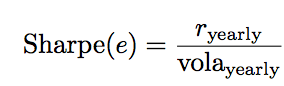
Sharpe ratio - the ratio of annual profit to annual volatility

Historical data for the competition includes approximately 3,800 trading days (data on price and trading volume) from January 1, 2001 to the present. The information is presented for 27 different futures contracts, including currency, precious metals, agricultural products, etc. The data includes the values ​​of the maximum, minimum price of the day, as well as the opening, closing and trading volumes for the period.

On each trading day, the rules of the competition allow the strategy to use as input data information about the previous 504 trading periods (which gives a vector of 2520 elements).

Montag suggested that it would be more effective to predict the future price and volatility of each futures contract independently of each other, using only data on their past behavior.

Algorithms

To predict the volatility and performance of trades, Montag used four regression algorithms:

• Linear and regularized regression (proprietary);
• Neural networks (using the MATLAB Neural Networks tool);
• Random forest (using the MATLAB Tree-Bagger function);
• Gradient booster of decision tree (GBM package for R).

The problem of predicting volatility was much simpler than the prediction of profit.

For each of the tasks, two data sets were used - a training set consisting of 9424 examples (80% of the available data) and a test set of 2356 examples (20% of the data). The distribution of training and test sets was chronological - training examples contained 80% of the initial data, and test examples consisted of 20% of the latest data.

results

Before starting to compare the performance of different machine learning algorithms, the researcher made a sample using linear regression:

Algorithm	Training r 2	CV r 2	Test r 2
PCA (82)	0.631	0.490	0.473
TI (18)	0.710	0.645	0.637
TI (7)	0.713	0.647	0.639

Here PCA is the principal component method , and TI is the technical indicators. The numbers in parentheses represent the dimensions of the feature vector.

After analyzing the main components reduced to 250 elements and the normalized vector, the optimal number of main components was obtained - 82. However, the use of linear regression, which uses the vector of all technical indicators of 18 elements, made it possible to achieve better results, and as a result, Montagu found seven technical parameters indicators, the use of which allows to further improve the results.

The table below provides information on the performance of the four algorithms in the field of volatility prediction using 7 indicators.

Algorithm	Training r 2	CV r 2	Test r 2
Lr	0.713	0.647	0.639
Nn	0.734	0.660	0.632
RF	0.731	0.664	0.649
GBM	0.701	0.666	0.638

Here LR is linear regression, NN is neural networks, RF is a random forest, GBM is a gradient boost of the decision tree. The best results were achieved using the random forest algorithm.

Below are the results of the effectiveness of the prediction of profit:

Algorithm	Training r 2	CV r 2	Test r 2
RR	0.169	0.142	0.138
Nn	0.088	0.013	-0.088
RF	0.236	0.069	-0.102
GBM	0.328	0.154	0.028

Here, RR is a regularized regression (which turned out to be the most effective), and the other abbreviations are identical to those used above. Negative values ​​correspond to the “short sale”.

To use the predictions of volatility and profit, Montag created a three-parameter trading algorithm that compares the expected profit with the predicted volatility, and uses the resulting value as the desired distribution of the portfolio.

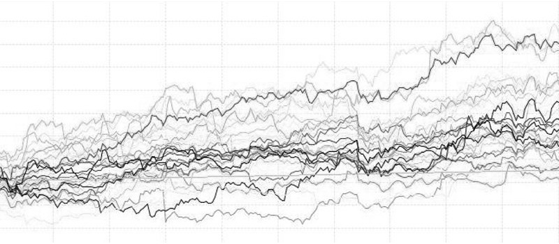
The graph below shows the performance of this strategy - it managed to achieve an annual profit of 6.63%, with an annual volatility of 5.58% and a Sharpe ratio of 1.18.



However, using only the first half of the available historical data, the strategy showed a Sharpe ratio of 1.33, while with a sample that included only the second part of the data, this number was much lower - 0.73. This fact indicates that you should not expect the same good performance strategy, both in the past and in the future, but you can count on a certain productivity.

According to Investopedia , a Sharpe ratio of 1 or higher is considered a good indicator, 2 or higher is very good, and 3 or higher is excellent. The strategies obtained using the above methods could show the maximum Sharpe ratio of 1.2 — on historical data, and much less for future data.

Despite the fact that these strategies have shown a profit, the likelihood that in real trading their Sharpe ratio will rise above one is not very large.