Visualization of static and dynamic networks on R, part 7, the last

In the first part :

• network visualization: why? how?
• visualization parameters
• best practices - aesthetics and performance
• data formats and preparation
• description of the data sets used in the examples
• getting started with igraph

In the second part : colors and fonts in graphs R.

In the third part: the parameters of graphs, vertices and edges.

In the fourth part: network placement.
')
In the fifth part: the emphasis on the properties of the network, vertices, edges, paths.

In the sixth part: interactive visualization of networks, other ways of representing the network.

In this part: animated visualization of networks, the evolution of the network over time.

Interactive and animated network visualization

Interactive 3D Networks in R

Now it is becoming easier to export R graphics to html / javascript. There are many libraries, such as rcharts and htmlwidgets , which are useful when creating web graphs directly from R. We look at the networkD3 library, which, as the name implies, creates interactive visualizations of networks using the D3 javascript library.

It should be understood that visualizations created using networkD3 are most useful as a starting point for further work. If you know a little javascript, you can use them as a first step and change them until you get the desired result.

If you do not have the networkD3 library, install it:

 install.packages("networkD3") 

The data used by this library is a standard list of edges with a couple of small changes. In order for everything to work, it is necessary that the identifiers of the vertices are numeric and start from scratch. An easy way to achieve this is to turn our literal identifiers into a factor variable, the result obtained is a number, and to ensure that the numbering is from zero by subtracting one.

 library(networkD3) el <- data.frame(from=as.numeric(factor(links$from))-1, to=as.numeric(factor(links$to))-1 ) 

Vertices must be in the same order as the source column in the links:

 nl <- cbind(idn=factor(nodes$media, levels=nodes$media), nodes) 

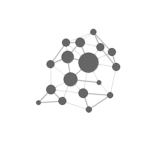
Now you can create an interactive presentation. The Group parameter is used to color the vertices. Nodesize is not the size of the vertex, as one might think, but the column number in the vertex data that needs to be used to set the size. The charge parameter controls repulsion (less than zero) or attraction (more than zero).

 forceNetwork(Links = el, Nodes = nl, Source="from", Target="to", NodeID = "idn", Group = "type.label",linkWidth = 1, linkColour = "#afafaf", fontSize=12, zoom=T, legend=T, Nodesize=6, opacity = 0.8, charge=-300, width = 600, height = 400) 

Simple animation of graphs in R

If you have already installed ndtv, you should also have an animation package. If not, now is the time to install it - install.packages('animation') . Note that this package allows you to easily create different (not necessarily related to networks) animations in R. This works like this: several graphs are created, which are then combined into a GIF.

The catch here is the following: in order for it to work, you need not only the R package, but also a special ImageMagick program.

 library(animation) library(igraph) ani.options("convert") # ,   ,   ImageMagick #   ,      . ani.options(convert="C:/Program Files/ImageMagick-6.8.8-Q16/convert.exe") 

Now we will create 4 network graphics (the same as before), only this time within the saveGIF . The animation interval is set by the interval parameter, the movie.name parameter sets the name of the gif file.

 l <- layout.fruchterman.reingold(net) saveGIF( { col <- rep("grey40", vcount(net)) plot(net, vertex.color=col, layout=l) step.1 <- V(net)[media=="Wall Street Journal"] col[step.1] <- "#ff5100" plot(net, vertex.color=col, layout=l) step.2 <- unlist(neighborhood(net, 1, step.1, mode="out")) col[setdiff(step.2, step.1)] <- "#ff9d00" plot(net, vertex.color=col, layout=l) step.3 <- unlist(neighborhood(net, 2, step.1, mode="out")) col[setdiff(step.3, step.2)] <- "#FFDD1F" plot(net, vertex.color=col, layout=l) }, interval = .8, movie.name="network_animation.gif" ) detach(package:igraph) detach(package:animation 

Interactive networks with ndtv-d3

Interactive graphics static networks

In this section, we will create more complex visualizations with the ndtv package. To create animations do not need additional software. If you want to save animations as video files (see ?saveVideo ), you need the FFmpeg video converter. To find out which installer is suitable for your OS, run ?install.ffmpeg . In order to use all available locations, you also need Java.

 install.packages("ndtv", dependencies=T) 

Since this package is part of Statnet, it will accept objects from the network package, like the one we created earlier.

 library(ndtv) net3 

Most of the parameters have intuitive names ( bg is the background color of the graphic). Two new parameters that were not previously used - vertex.tooltip and edge.tooltip . They contain information that can be seen by hovering the mouse over a network element. Note that the parameters for tooltips accept html tags - for example, use the line break tag - <br> . The launchBrowser parameter launchBrowser R to open the resulting visualization file ( filename ) in the browser.

 render.d3movie(net3, usearrows = F, displaylabels = F, bg="#111111", vertex.border="#ffffff", vertex.col = net3 %v% "col", vertex.cex = (net3 %v% "audience.size")/8, edge.lwd = (net3 %e% "weight")/3, edge.col = '#55555599', vertex.tooltip = paste("<b>Name:</b>", (net3 %v% 'media') , "<br>", "<b>Type:</b>", (net3 %v% 'type.label')), edge.tooltip = paste("<b>Edge type:</b>", (net3 %e% 'type'), "<br>", "<b>Edge weight:</b>", (net3 %e% "weight" ) ), launchBrowser=F, filename="Media-Network.html", output.mode='inline') 

Network evolution animation

Animated visualizations are a good way to show the time evolution of a small or medium sized network. At the moment, ndtv is the best R package designed for this purpose - especially after the three-dimensional visualization feature was recently added.

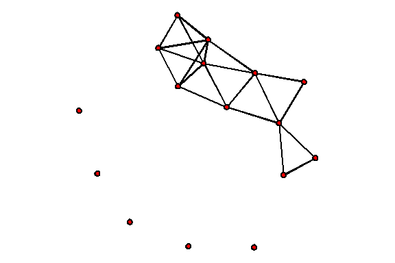
In order to work with network animation in ndtv , you need to understand the dynamic format of the Statnet network, implemented in the networkDynamic package. Let's look at one of the data sets included in the package as an example:

 data(short.stergm.sim) short.stergm.sim head(as.data.frame(short.stergm.sim)) 

 ## onset terminus tail head onset.censored ## 1 0 1 3 5 FALSE ## 2 10 20 3 5 FALSE ## 3 0 25 3 6 FALSE ## 4 0 1 3 9 FALSE ## 5 2 25 3 9 FALSE ## 6 0 4 3 11 FALSE 

 ## terminus.censored duration edge.id ## 1 FALSE 1 1 ## 2 FALSE 10 1 ## 3 FALSE 25 2 ## 4 FALSE 1 3 ## 5 FALSE 23 3 ## 6 FALSE 4 4 

Here we see a list of edges. Each edge comes from a vertex whose identifier is in the tail column and enters a vertex with an identifier in the head column. An edge exists from the onset timestamp to the terminus timestamp. Onset and terminus, marked censored , mean the beginning and end of the observation of the network, and not the actual formation and disappearance of connections.

You can easily build a network without taking into account its temporal component (by combining all the vertices and edges ever presented):

 plot(short.stergm.sim) 

Construct a network at time 1:

 plot( network.extract(short.stergm.sim, at=1) ) 

We construct vertices and edges active from the first to the fifth time instant:

 plot( network.extract(short.stergm.sim, onset=1, terminus=5, rule="all") ) 

We construct vertices and edges active from the first to the tenth time instant:

 plot( network.extract(short.stergm.sim, onset=1, terminus=10, rule="any") ) 

Let's make a short three-dimensional network animation from the example:

 render.d3movie(short.stergm.sim,displaylabels=TRUE) 

Now we are ready to create and animate our own dynamic network. The dynamic network object can be obtained in several ways: from a set of networks / matrices representing different points in time, from matrices / datasets with lists of vertices and edges, which indicate when they are active or when they change state. More information is available in ?networkDynamic .

Add a time component to our media example. The code below takes a time interval from 0 to 50 and makes the vertices of the network active all the time. Edges appear one after another, each active from the moment of appearance until the 50th time point. Create such a network using networkDynamic , the time for the vertices is node.spelss , for the edges — edge.spells .

 vs <- data.frame(onset=0, terminus=50, vertex.id=1:17) es <- data.frame(onset=1:49, terminus=50, head=as.matrix(net3, matrix.type="edgelist")[,1], tail=as.matrix(net3, matrix.type="edgelist")[,2]) net3.dyn <- networkDynamic(base.net=net3, edge.spells=es, vertex.spells=vs) 

If you just try to build a networkDynamic-network, you get a combined network for the entire observation period, initial example with the media.

 plot(net3.dyn, vertex.cex=(net3 %v% "audience.size")/7, vertex.col="col") 

One way to show the evolution of the network over time is static pictures for different points in time. Although you can generate them one by one, as we did above, ndtv offers an easier way. The team for this is the filmstrip . As in the par() function that controls the parameters of graphs R, here mfrow sets the number of rows and columns in a table into several graphs.

 filmstrip(net3.dyn, displaylabels=F, mfrow=c(1, 5), slice.par=list(start=0, end=49, interval=10, aggregate.dur=10, rule='any')) 

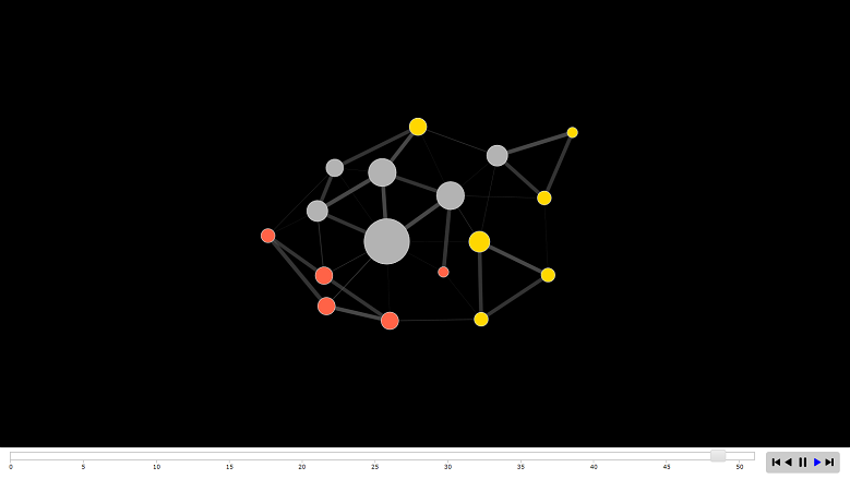
You can calculate in advance the coordinates of the animation (otherwise they are considered at the time of creation of the animation). Here, animation.mode is a location algorithm — one of “kamadakawai”, “MDSJ”, “Graphviz” and “use Attribute” (user-defined coordinates).

 compute.animation(net3.dyn, animation.mode = "kamadakawai", slice.par=list(start=0, end=50, interval=1, aggregate.dur=1, rule='any')) render.d3movie(net3.dyn, usearrows = F, displaylabels = F, label=net3 %v% "media", bg="#ffffff", vertex.border="#333333", vertex.cex = degree(net3)/2, vertex.col = net3.dyn %v% "col", edge.lwd = (net3.dyn %e% "weight")/3, edge.col = '#55555599', vertex.tooltip = paste("<b>Name:</b>", (net3.dyn %v% "media") , "<br>", "<b>Type:</b>", (net3.dyn %v% "type.label")), edge.tooltip = paste("<b>Edge type:</b>", (net3.dyn %e% "type"), "<br>", "<b>Edge weight:</b>", (net3.dyn %e% "weight" ) ), launchBrowser=T, filename="Media-Network-Dynamic.html", render.par=list(tween.frames = 30, show.time = F), plot.par=list(mar=c(0,0,0,0)), output.mode='inline' ) 

In addition to dynamic vertices and edges, ndtv accepts dynamic parameters. You could add them to the es and vs datasets above. Moreover, the build function can apply special parameters and create dynamic arguments directly in the process. For example, function (slice) {some calculations with slice} will perform actions in the current time slice, thereby allowing the parameters to be dynamically changed. Pay attention to the size of the vertices below:

 compute.animation(net3.dyn, animation.mode = "kamadakawai", slice.par=list(start=0, end=50, interval=4, aggregate.dur=1, rule='any')) render.d3movie(net3.dyn, usearrows = F, displaylabels = F, label=net3 %v% "media", bg="#000000", vertex.border="#dddddd", vertex.cex = function(slice){ degree(slice)/2.5 }, vertex.col = net3.dyn %v% "col", edge.lwd = (net3.dyn %e% "weight")/3, edge.col = '#55555599', vertex.tooltip = paste("<b>Name:</b>", (net3.dyn %v% "media") , "<br>", "<b>Type:</b>", (net3.dyn %v% "type.label")), edge.tooltip = paste("<b>Edge type:</b>", (net3.dyn %e% "type"), "<br>", "<b>Edge weight:</b>", (net3.dyn %e% "weight" ) ), launchBrowser=T, filename="Media-Network-even-more-Dynamic.html", render.par=list(tween.frames = 15, show.time = F), output.mode='inline')