Hands-On Programming With R - Garrett Grolemund
Full translation of the book Hands-on Programming With R - Garrett Grolemund into Russian.
Enjoy reading!
Studying programming is very important if we want to learn how to analyze data. Without a doubt, “data science” should be performed on modern computers, but we have a choice between using graphical interfaces of ready-made software products and programming in existing languages. Garrett and I both are convinced that programming in the modern world is an essential and vital skill for those who constantly work with data. The graphical interface, despite all its comforts, prevents good data analysis:
')
Do not be afraid to program! Anyone can learn how to program with the right motivation, and this book is organized to keep you motivated. This is not a reference; This is a book about three issues. The book will guide you through the fascinating basics of the R language and even allow you to look into the next level of complexity. Real tasks are the best way to learn, because you don’t memorize functions out of context, you learn them to solve problems from the real world. You will be trained in completing tasks.
In the process of learning programming, you will be disappointed / upset. Learning a new language takes time and patience. It is worth remembering that disappointment is a natural feeling, the appearance of which must be fixed and perceived as a positive moment. Frustration is the way the brain is lazy, diverting your attention to things that are simpler and more fun. If you really want to get in good shape, you must continue to work, despite all the pain in the body. If you really want to learn how to program, then you need to force the brain to concentrate and get involved in the work. Remember this moment, because it means that you have started stretching - stretching yourself. Every day, push yourself to move forward and soon you will become a confident programmer.
We hope that reading our joint work with Garrett will bring you pleasure.
This book will teach you how to program in the R language. Your journey will begin with data loading and end with the writing of your own functions (which will easily surpass the functions of other users of the R language). However, this is no ordinary introduction to the R language. I want to help you become datologists (analysts) , as well as computer specialists, so this book will focus on programming skills for solving problems in datology .
The chapters in the book are divided and sorted in order of increasing complexity of the implementation of three practical projects. I chose these projects for two reasons. First, they display the broad capabilities of the R language. You will learn how to load data, assemble and parse objects, write your own functions and use all the tools available in R, such as if-else constructions, for loops, classes, packages, debugging tools. Projects also teach you to write vectorized code that uses all the power of R.
However, most importantly, projects will teach you how to solve logical problems in data science - and there are really a lot of problems! Working with data we need to store them, retrieve and modify large arrays of values without introducing errors. In the process of learning, we will learn not only to program in R, but also to use our programmer skills to maintain our work as a datologist.
Not every programmer needs to be a datologist, so not every programmer will find this book useful. You will find this book useful for yourself if you belong to one of the following categories:
One of the big disappointments in this book is the lack of references and consideration of the use of the R language in traditional applications - models and graphs. I perceive R as a typical programming language. Why such a narrow focus? R was designed as a tool to help professionals analyze data. It has many excellent features for graphing and modeling. As a result, a lot of extras use R as if it were ordinary software — they only learn the functions they need, but they don’t pay attention to the rest.
Computers allow you to collect, manipulate, visualize arrays of data and all this with a speed that would surprise yesterday’s scientists. In short, computers give you a scientific super power! However, in order to learn how to use these super powers, you will need to acquire programming skills.
As a data scientist and programmer, you can enhance your skills in the following areas:
Computers can solve all these problems quickly and accurately, which allows your mind to do what it does best: make decisions and give meaning.
Sounds amazing? Wonderful! Let's get started
Being a college student I wanted to go to Las Vegas. At that time, I was sure that knowing the statistics would help me to make a big win. If this is what prompted you to study the science of data, then I ask you to sit down. I have bad news for you. In the long run, even a statistician will lose a lot of money at the casino. And all because in every single game the chances of winning are greater than the casino. However, you can always find a loophole. You can make money - securely. All you need to do is become a casino owner.
Believe it or not, R can help you with that. Throughout the book, we will use R to create three virtual objects: a pair of dice that we can throw; a deck of cards that we can shuffle and hand out; slot machine in which we simulate a game from a real gaming terminal. After that, all you need to do is add some graphics and open a bank account (and get several state licenses), and you are in! Understand the rest of the details yourself.
Projects seem insignificant, but in reality each of them will allow you to look deep “under the hood” of R. After their completion, you will become an expert in the field of data analysis and processing. You will learn how to store data in computer memory, process it, convert it to another type, make transformations, etc. You will also learn how to write programs on R, which can then be used for data analysis and simulation.
If the simulation of slot machines (dice, cards) seems like child's play, then think about this: playing on slot machines is a process. Once you can simulate it, then you can simulate other processes. These projects provide specific examples of using the components of the R language: objects, data types, classes, notations, functions, environment variables, loops, conditional statements, vectorization. The first project will introduce you to the basics of the R language, which will further help you learn all of the above.
The first task is simple: write the code in R, which will simulate the throwing of two dice. After that, we will change the weights of the dice values so that you will win more :)
In this project you will learn how to:
Do not be afraid if you think that the information is too much and you will not have time to deal with it. These topics will be covered over 2 and 3 projects.
This chapter is an overview of the R language, which will allow you to start programming without delay. You will create two virtual dice that will generate random values. If you have not programmed before - do not be afraid, this chapter will teach you everything you need.
In order to simulate the dice it is necessary to describe their properties. We will not put a physical object into the computer, and if we place it, then it is unlikely that we will be able to collect it back, but we can store information about the object in the computer’s memory.
What information needs to be kept? A dice has six different “pieces” of useful information: the result of throwing a dice can be only one value out of 6 (1, 2, 3, 4, 5, 6). We can save this data as a set of integer values.
Let's see first with the preservation of these values, and then consider the method of "throwing" the dice.
Before you ask your computer to save certain values, you need to learn how to talk with it. And here R and RStudio already come to our aid. RStudio gives you the opportunity to talk with a computer, and R - the language you will speak. Run RStudio.
The RStudio interface is simple. Enter commands into the RStudio console, press Enter to execute them. The code you enter into the console is called a command , because it tells the computer to perform certain actions. The line on which the command is entered is called the command line . After you type something into the command line and press Enter, the computer executes this command and displays the result on the screen. Immediately after the result of the previous command, a new RStudio query line appears.
For example, if you type 1 + 1 and press Enter, RStudio displays:
You probably noticed [1] right before the results of the calculations. R just tells us that this is the first line of the resulting output.
Some commands return more than one value and they may take several lines. For example, the command 100: 130 returns 31 values; it creates a sequence of integers from 100 to 130. Note that the numbers in square brackets are displayed at the very beginning of the first and second lines of output. These values indicate that the second line starts with 26 values from the sequence. In most cases, you can ignore the values in square brackets:
The colon operator (:) returns all integer values between two numbers. This is an easy way to create integer sequences.
When does the compilation happen?
In some languages, such as C / Java / C ++ / FORTRAN, you need to convert readable code into machine code before you execute it. If you previously programmed in one of these languages, then you probably wonder if it is necessary to compile the code in R. Answer: no. R is a dynamic programming language, which means that R automatically interprets your code as soon as you run it.
If you enter an incomplete command and press Enter, R will display the continuation of the prompt for input - "+". Either complete the command or press Esc to abort it and start again:
If you enter a command that R cannot recognize, an error message will be displayed. If you ever see an error message, do not panic. R just informs you that he was unable to execute a specific command for some reason. You can then try another command on the following command line:
As soon as you feel free to work on the command line, you can do everything that the most advanced calculator does. For example, let's start with basic arithmetic:
R handles hashtags (#) in a special way. No command will be executed after the hashtag (#). This makes hashtags useful when commenting or documenting code. The hashtag is known in R as the “comment character”.
Cancel commands
Some commands in R can be executed for a long time. You can interrupt the execution with ctrl + c, but remember that the interruption of the command itself may take a long time.
Now that you know how to use R, let's create a virtual die. The operator ":", with which we have already met a few pages back, allows you to conveniently create a group of numbers from 1 to 6.
The ":" operator returns a vector , one-dimensional array of numbers:
This is how virtual dice look like! But do not be in a hurry to get upset, this is not all. Execution of the “1: 6” command only creates and displays an integer vector, but we do not save it anywhere. If we want to be able to reuse these numbers, then we need to save them somewhere. This will help us to create objects .
R allows you to store data in objects . What is an object ? Just the name that is used to refer to the stored data. For example, you can save data in objects a or b . In any place where R meets an object, it replaces it with a value stored inside, for example:
1. To create an object in R, create a name for it and use the "<-" symbol to save data. R will create an object, give it a name and save everything that is to the right of "<-".
2. When you ask R what is in “a”, then R displays the saved data on the next line.
3. You can also use the created objects in subsequent commands.
Another example, the code below creates a new object called die containing numbers from 1 to 6. To see what the object contains, just type the name of the object and press Enter.
After you have created an object, it will appear in the RStudio variable panel. In this part of the interface you can find all created objects since the launch of RStudio.
You can name objects in R as you wish, however there are several basic rules. First, the object name cannot begin with a digit. Secondly, the name cannot contain special characters - ^,!, $, @, +, -, /, *.
It is worth remembering that in R the Name and name variables are two different variables.
R overwrites any previously stored information in the object without any request for permission to perform this action. Therefore, it is good practice to avoid reusing existing variables:
Using the ls () function, you can get a list of variable names that are already in use:
You can also just look at the variables panel in RStudio to determine which variable names are already used and what data is stored in them.
Now you have a virtual dice that is stored in the computer's memory. At any time you can access it simply by typing die in the command line. What can you do with the dice? Enough. R will replace the object with its contents in any command. Therefore, for example, you can perform various arithmetic operations on the values of the dice. Mathematics is not so important when throwing a die, but when working with a lot of data will become an indispensable tool. Let's see how and what can be done:
If you are a big fan of linear algebra (and who is not?), Then you probably noticed that R does not always follow the rules of matrix multiplication. Instead, R uses per-element multiplication. When you work with a set of numbers, R will apply a specific operation to each element in the set separately. For example, when we launch die - 1 , then R subtracts a unit from each element in die .
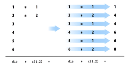
When using several vectors in operations, R first equalizes the lengths of the vectors and only then elementwise performs the operation itself. For example, when performing the operation die * die , R aligns the lengths of the two vectors, and then multiplies the first value from the first vector by the first value from the second vector, etc., until all the elements are multiplied. The result of this operation will be a new vector of the same length as the two multiplied vectors.
If you pass R two vectors of different lengths, then R will “repeat” / “loop” a vector of shorter length until it becomes equal in length to the larger vector. The change in the smaller vector is not a constant change (the source vector does not change), it is supplemented only for the duration of the operation. If the length of the larger vector is not a multiple of the length of the smaller vector, then R will issue a warning. This behavior is known as vector recycling and allows R to perform in-element operations:
By-element operations are extremely important in R, as they allow processing of groups of values in a specific order. When you begin to work with a variety of data, per-element operations will make sure that the data from one observation exactly matches the data from another observation. By-element operations also simplify the creation of eigenfunctions and programs on R.
However, do not think that R abandoned the traditional matrix work. You just need to use the right operator.
Use the % *% operator for the inner work, and % o% for the outer work.
You can also transpose the matrix using the t function and calculate its determinant using the det function.
Do not worry if you are not familiar with these features. Their description is simply found in the documentation, besides, in this book you will not need them.
Now that you have figured out how to perform math operations on the values of the die, let's see how we can program the throw (throwing the dice). To throw the dice you need something more magical than basic arithmetic; You will need to randomly select one of the dice values. But for this you need a function .
R initially contains many useful and surprising functions that you can use for such tasks as, for example, generating a random sample. For example, you can round the number with the round () function, or calculate the factorial of the number with the factorial () function. Using functions is quite simple. You write the name of the function you want to use, and in parentheses the data over which you need to perform the calculations:
The data you pass to a function is called a function argument. The argument can be as raw data, objects or other functions of R. In the latter case, R will perform functions in the order of decreasing their nesting.
To our happiness, there is a function in R that can help us with the implementation of the die roll. You can simulate a die roll using the sample function. The sample function takes two arguments: the vector x and the name parameter size . The sample function returns the size of elements from the x vector.
To simulate a die roll and get one numeric value as a result, set x to die and highlight / select one random element.
Each time you start you will have a different value:
The set of functions in R takes several arguments that help it perform its stated task. You can pass as many arguments to the function as long as each of them is separated by a comma.
You could have noticed that I assigned the values die and 1 to the specific named arguments of the sample function x and size . Each argument in the R function has its own name. You can specify which values to assign to which arguments, as was shown in the previous example. It becomes extremely convenient to do when you pass multiple parameters into one function; Named arguments eliminate errors with passing the wrong data to the wrong arguments. The use of names is the solution of each and is not mandatory. You may notice that R users often do not specify the name of the first argument of the function. The previous code can be rewritten as follows:
Very often, the name of the first argument is not very meaningful, and most often it is clear what data must be passed to the function first.
How do you know which argument names to use? If you try to use names that the function does not expect, you will most likely get an error message:
If you doubt which argument names can be passed to a function, you can use the args function, which will list all possible named arguments of a particular function. To do this, put the name of the function in parentheses as an argument - args (the name of the function) . For example, you see that the round function takes two arguments — one with the name x , the second with the name digits :
Did you notice that the digits name argument in the round function is set to 0 by default? Often functions in R accept optional parameters, such as digits . These arguments are considered optional because they have already been assigned a default value. You can pass a new value for such a parameter if you want, or use the default provided. For example, round rounds clean to the nearest 0 decimal values by default. To overwrite the default, pass in the new:
You should specify named arguments after the first or second argument of the function when calling a function with multiple arguments. Why? First, it will help you and other developers understand the code. It is often clear what the transmitted data refers to in the first and second arguments. However, you will need a phenomenal memory to remember all subsequent argument names for all existing functions in R. Secondly, and more importantly, this will avoid annoying errors.
If you do not use named arguments, then R will automatically match the arguments with the parameters in the order in which you passed them. For example, in the example below, the first die value will be assigned to the variable x , the second value 1 will be assigned to size .
The more arguments you pass, the greater the likelihood of diverging the order in which arguments are passed. As a result, values can be passed to the wrong arguments. Named arguments exclude such errors. R will always correctly assign a value to a named argument, regardless of the order in which they follow.
If you set size = 2, then you almost modeled the dice rolls. Before you run this code, think a minute, what’s wrong?
sample returns two numbers, one for each die:
I said “almost” because this method works a bit differently than we expect. If we run the code above several times, we note that the second value will never coincide with the first, which means we will never be able to throw two triples or two sixes. What's happening?
By default, sample samples without recovery . To figure out what this means, imagine that sample places all die values in an urn (basket). Then sample randomly fetches the values one by one from the basket for building the sample. After sample has used the selected value, it is not returned back and cannot be reused. Therefore, if the value of 6 falls for the first time, then the second time it will no longer be able to drop; 6 is no longer in the basket.
A side effect of this behavior is the dependence of subsequent shots from previous ones. In the real world, however, when you roll a pair of dice, each dice is independent of the others. If 6 falls on the first die, this does not prevent the loss of 6 and on the second die. You can recreate this behavior in sample by simply passing the optional argument replace = TRUE .
The argument replace = TRUE changes the operation of the sample function. Our initial basket example is a good way to show how a sample works with and without replacement / repair. sample with replacement after selecting an arbitrary value from the basket returns it back. As a result, we have achieved the desired effect.
Sampling with recovery is an easy way to create independent random samples (blah blah blah ...). Each value in your sample will be a sample of size 1 that does not depend on other values. The correct way to simulate a roll of a pair of dice:
You can praise yourself; you have just implemented your first simulation on R! You now have a method to simulate a roll of a die. If you want to add the dropped dice values, you can simply pass the result of the sample to the sum function.
What happens if you call dica several times? Will R generate a new pair of values for each roll? Let's try:
Not. Each time you call dica in R, the values that were once stored in this object will be displayed as a result.
However, it would be logical to have an object that would be able to generate a new pair of values with each simulation of the throw. You can implement this by writing your own R function.
Recall that you already have a working code on R that simulates a roll of two dice:
You can reprint this code into the console R each time you want to make a new dice roll. However, this is quite a strange way. It would be much more convenient to use this code once in our function and then call it. This we now do. We are going to write the roll function, which you can use to simulate a roll of a virtual dice. When you are done, the function will work as follows: each time roll () is called, R will return the sum of the values of the two rolled dice.
Functions may seem magical and bizarre, but they are nothing more than the type of object in R. Functions do not contain data, but code. This code is stored in a format that allows it to be reused in other programs.
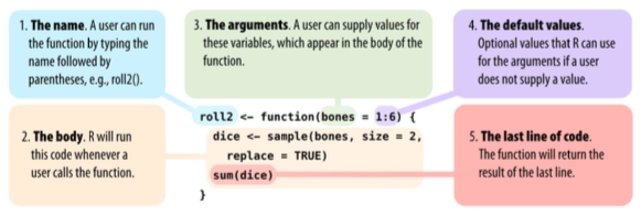
Each function in R consists of three main parts: a name, a body, a list of arguments. To write your own function, you need to create these three parts and store them in an object using the function () function :
function will create a function from any R code that you place between the opening and closing curly braces. For example, you can transfer all of your previous dice-throw code into a function:
After opening the curly bracket, the command line R will wait for the remaining commands to enter until it finds the closing curly bracket of the function.
Remember to save the result of the function function to an R object. This object will now become a function. To use the new function, enter the object name, opening and closing parentheses:
You can count the parentheses after the object name as a trigger that runs the code inside the object for execution. If you enter a function name without parentheses, then R will show you directly the code stored in the function object:
The code that you put into a function is called the function body . When a function is executed in R, R will execute all the code that is in the function body and return the value that will be calculated on the last line. If the last line does not return any value, it means that your function will not return anything.
Here is the code that displays the result after the execution on the last line:
But the code that does not display the results after the execution on the last line:
Notice the difference? These lines of code do not return a value to the command line; they store values in the object.
What would happen if we removed one line from our code and renamed the die variable to bones :
If you now call the roll2 function , you will get an error message. For the function to work correctly, a bones object is needed , but such an object does not exist:
You can pass bones as an argument to the roll2 function . To do this, you must specify the name of the argument in parentheses in the function declaration:
Now the roll2 function will work if you pass bones to it . You can use this to throw away different types of dice.
Remember that we are throwing two dice:
Note that when you call roll2, it will still return an error if you do not pass values to the bones argument .
You can prevent this error from appearing on such a call by setting the default bones argument . You can do this as follows:
Now you can safely call the roll2 function to simulate a roll of two dice:
You can pass an unlimited number of arguments to your functions. To do this, list their names separated by commas between parentheses when declaring a function. Each time the function is started, R will automatically replace the argument name with the value that was passed to it. If no value was passed, then R will use the default value.
Summing up, function is used to declare eigenfunctions in R. The function code is placed between two curly braces. Arguments are specified after the function name, separated by commas between two parentheses.
After you have written your function, R will perceive it as any other function. Just imagine how useful and convenient this is. Have you ever tried to create a new function for Excel and add it to the panel with the menu? Or a new type of animation as a new option in PowerPoint? When you work with a programming language, all this becomes available to you. While learning the R language, you will learn how to create new, customizable, reproducible tools for any occasion. In part 3, we take a closer look at the functions.
Remember:
To be continued…
Enjoy reading!
Foreword
Studying programming is very important if we want to learn how to analyze data. Without a doubt, “data science” should be performed on modern computers, but we have a choice between using graphical interfaces of ready-made software products and programming in existing languages. Garrett and I both are convinced that programming in the modern world is an essential and vital skill for those who constantly work with data. The graphical interface, despite all its comforts, prevents good data analysis:
')
- Reproducibility (ability to recreate previous results)
- Automation (the ability to quickly get results when data changes)
- Communication (code is just a text, so it is easier to understand. When learning, it is very easy to get help, be it Google Groups, email, Stack Overflow, etc.)
Do not be afraid to program! Anyone can learn how to program with the right motivation, and this book is organized to keep you motivated. This is not a reference; This is a book about three issues. The book will guide you through the fascinating basics of the R language and even allow you to look into the next level of complexity. Real tasks are the best way to learn, because you don’t memorize functions out of context, you learn them to solve problems from the real world. You will be trained in completing tasks.
In the process of learning programming, you will be disappointed / upset. Learning a new language takes time and patience. It is worth remembering that disappointment is a natural feeling, the appearance of which must be fixed and perceived as a positive moment. Frustration is the way the brain is lazy, diverting your attention to things that are simpler and more fun. If you really want to get in good shape, you must continue to work, despite all the pain in the body. If you really want to learn how to program, then you need to force the brain to concentrate and get involved in the work. Remember this moment, because it means that you have started stretching - stretching yourself. Every day, push yourself to move forward and soon you will become a confident programmer.
We hope that reading our joint work with Garrett will bring you pleasure.
Introduction
This book will teach you how to program in the R language. Your journey will begin with data loading and end with the writing of your own functions (which will easily surpass the functions of other users of the R language). However, this is no ordinary introduction to the R language. I want to help you become datologists (analysts) , as well as computer specialists, so this book will focus on programming skills for solving problems in datology .
The chapters in the book are divided and sorted in order of increasing complexity of the implementation of three practical projects. I chose these projects for two reasons. First, they display the broad capabilities of the R language. You will learn how to load data, assemble and parse objects, write your own functions and use all the tools available in R, such as if-else constructions, for loops, classes, packages, debugging tools. Projects also teach you to write vectorized code that uses all the power of R.
However, most importantly, projects will teach you how to solve logical problems in data science - and there are really a lot of problems! Working with data we need to store them, retrieve and modify large arrays of values without introducing errors. In the process of learning, we will learn not only to program in R, but also to use our programmer skills to maintain our work as a datologist.
Not every programmer needs to be a datologist, so not every programmer will find this book useful. You will find this book useful for yourself if you belong to one of the following categories:
- You already use R as a statistical tool, but want to learn how to write your own functions and simulations on R.
- You want to learn how to program and see the point in learning a language able to work with data
One of the big disappointments in this book is the lack of references and consideration of the use of the R language in traditional applications - models and graphs. I perceive R as a typical programming language. Why such a narrow focus? R was designed as a tool to help professionals analyze data. It has many excellent features for graphing and modeling. As a result, a lot of extras use R as if it were ordinary software — they only learn the functions they need, but they don’t pay attention to the rest.
Part number 1
Project 1: weighted dice
Computers allow you to collect, manipulate, visualize arrays of data and all this with a speed that would surprise yesterday’s scientists. In short, computers give you a scientific super power! However, in order to learn how to use these super powers, you will need to acquire programming skills.
As a data scientist and programmer, you can enhance your skills in the following areas:
- Memorize (store) large data arrays
- Request data
- Make complex calculations on large amounts of data
- Perform repetitive tasks without getting bored
Computers can solve all these problems quickly and accurately, which allows your mind to do what it does best: make decisions and give meaning.
Sounds amazing? Wonderful! Let's get started
Being a college student I wanted to go to Las Vegas. At that time, I was sure that knowing the statistics would help me to make a big win. If this is what prompted you to study the science of data, then I ask you to sit down. I have bad news for you. In the long run, even a statistician will lose a lot of money at the casino. And all because in every single game the chances of winning are greater than the casino. However, you can always find a loophole. You can make money - securely. All you need to do is become a casino owner.
Believe it or not, R can help you with that. Throughout the book, we will use R to create three virtual objects: a pair of dice that we can throw; a deck of cards that we can shuffle and hand out; slot machine in which we simulate a game from a real gaming terminal. After that, all you need to do is add some graphics and open a bank account (and get several state licenses), and you are in! Understand the rest of the details yourself.
Projects seem insignificant, but in reality each of them will allow you to look deep “under the hood” of R. After their completion, you will become an expert in the field of data analysis and processing. You will learn how to store data in computer memory, process it, convert it to another type, make transformations, etc. You will also learn how to write programs on R, which can then be used for data analysis and simulation.
If the simulation of slot machines (dice, cards) seems like child's play, then think about this: playing on slot machines is a process. Once you can simulate it, then you can simulate other processes. These projects provide specific examples of using the components of the R language: objects, data types, classes, notations, functions, environment variables, loops, conditional statements, vectorization. The first project will introduce you to the basics of the R language, which will further help you learn all of the above.
The first task is simple: write the code in R, which will simulate the throwing of two dice. After that, we will change the weights of the dice values so that you will win more :)
In this project you will learn how to:
- Use R and RStudio
- Execute commands on R
- Create objects
- Write your own functions and scripts
- Download and use packages
- Generate test data
- Build graphics
- Use documentation
Do not be afraid if you think that the information is too much and you will not have time to deal with it. These topics will be covered over 2 and 3 projects.
Chapter 1
Basics
This chapter is an overview of the R language, which will allow you to start programming without delay. You will create two virtual dice that will generate random values. If you have not programmed before - do not be afraid, this chapter will teach you everything you need.
In order to simulate the dice it is necessary to describe their properties. We will not put a physical object into the computer, and if we place it, then it is unlikely that we will be able to collect it back, but we can store information about the object in the computer’s memory.
What information needs to be kept? A dice has six different “pieces” of useful information: the result of throwing a dice can be only one value out of 6 (1, 2, 3, 4, 5, 6). We can save this data as a set of integer values.
Let's see first with the preservation of these values, and then consider the method of "throwing" the dice.
User Interface R
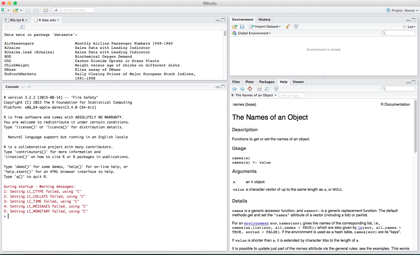
Before you ask your computer to save certain values, you need to learn how to talk with it. And here R and RStudio already come to our aid. RStudio gives you the opportunity to talk with a computer, and R - the language you will speak. Run RStudio.
The RStudio interface is simple. Enter commands into the RStudio console, press Enter to execute them. The code you enter into the console is called a command , because it tells the computer to perform certain actions. The line on which the command is entered is called the command line . After you type something into the command line and press Enter, the computer executes this command and displays the result on the screen. Immediately after the result of the previous command, a new RStudio query line appears.
For example, if you type 1 + 1 and press Enter, RStudio displays:
> 1+1 [1] 2 > You probably noticed [1] right before the results of the calculations. R just tells us that this is the first line of the resulting output.
Some commands return more than one value and they may take several lines. For example, the command 100: 130 returns 31 values; it creates a sequence of integers from 100 to 130. Note that the numbers in square brackets are displayed at the very beginning of the first and second lines of output. These values indicate that the second line starts with 26 values from the sequence. In most cases, you can ignore the values in square brackets:
> 100:130 [1] 100 101 102 103 104 105 106 107 108 109 110 111 112 113 114 115 116 117 118 119 120 121 122 123 124 [26] 125 126 127 128 129 130 > The colon operator (:) returns all integer values between two numbers. This is an easy way to create integer sequences.
When does the compilation happen?
In some languages, such as C / Java / C ++ / FORTRAN, you need to convert readable code into machine code before you execute it. If you previously programmed in one of these languages, then you probably wonder if it is necessary to compile the code in R. Answer: no. R is a dynamic programming language, which means that R automatically interprets your code as soon as you run it.
If you enter an incomplete command and press Enter, R will display the continuation of the prompt for input - "+". Either complete the command or press Esc to abort it and start again:
> 5- + 1 [1] 4 > If you enter a command that R cannot recognize, an error message will be displayed. If you ever see an error message, do not panic. R just informs you that he was unable to execute a specific command for some reason. You can then try another command on the following command line:
> 3 % 6 Error: unexpected input in "3 % 6" > As soon as you feel free to work on the command line, you can do everything that the most advanced calculator does. For example, let's start with basic arithmetic:
> 2 * 3 [1] 6 > 4 - 1 [1] 3 > 6 / (4 - 1) [1] 2 > R handles hashtags (#) in a special way. No command will be executed after the hashtag (#). This makes hashtags useful when commenting or documenting code. The hashtag is known in R as the “comment character”.
Cancel commands
Some commands in R can be executed for a long time. You can interrupt the execution with ctrl + c, but remember that the interruption of the command itself may take a long time.
Now that you know how to use R, let's create a virtual die. The operator ":", with which we have already met a few pages back, allows you to conveniently create a group of numbers from 1 to 6.
The ":" operator returns a vector , one-dimensional array of numbers:
> 1:6 [1] 1 2 3 4 5 6 This is how virtual dice look like! But do not be in a hurry to get upset, this is not all. Execution of the “1: 6” command only creates and displays an integer vector, but we do not save it anywhere. If we want to be able to reuse these numbers, then we need to save them somewhere. This will help us to create objects .
Objects
R allows you to store data in objects . What is an object ? Just the name that is used to refer to the stored data. For example, you can save data in objects a or b . In any place where R meets an object, it replaces it with a value stored inside, for example:
> a <- 1 > a [1] 1 > a + 2 [1] 3 1. To create an object in R, create a name for it and use the "<-" symbol to save data. R will create an object, give it a name and save everything that is to the right of "<-".
2. When you ask R what is in “a”, then R displays the saved data on the next line.
3. You can also use the created objects in subsequent commands.
Another example, the code below creates a new object called die containing numbers from 1 to 6. To see what the object contains, just type the name of the object and press Enter.
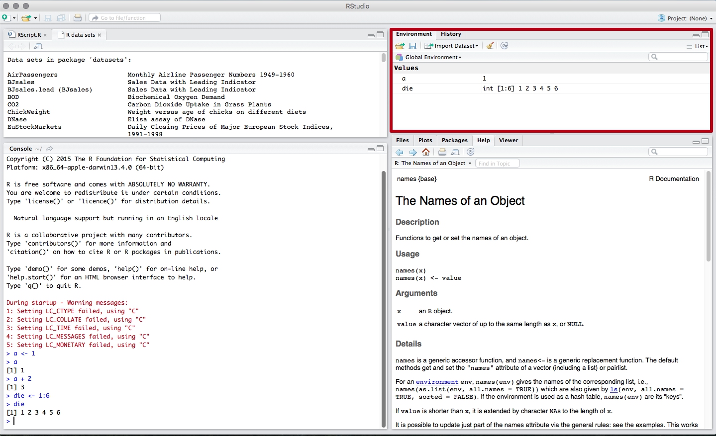
> die <- 1:6 > die [1] 1 2 3 4 5 6 After you have created an object, it will appear in the RStudio variable panel. In this part of the interface you can find all created objects since the launch of RStudio.
You can name objects in R as you wish, however there are several basic rules. First, the object name cannot begin with a digit. Secondly, the name cannot contain special characters - ^,!, $, @, +, -, /, *.
| Correct names | Wrong names |
|---|---|
| my_var | ^ mean |
| FOO | 2nd |
| b | ! bad |
It is worth remembering that in R the Name and name variables are two different variables.
R overwrites any previously stored information in the object without any request for permission to perform this action. Therefore, it is good practice to avoid reusing existing variables:
> my_number <- 1 > my_number [1] 1 > my_number <- 999 > my_number [1] 999 Using the ls () function, you can get a list of variable names that are already in use:
> ls() [1] "a" "die" "my_number" You can also just look at the variables panel in RStudio to determine which variable names are already used and what data is stored in them.
Now you have a virtual dice that is stored in the computer's memory. At any time you can access it simply by typing die in the command line. What can you do with the dice? Enough. R will replace the object with its contents in any command. Therefore, for example, you can perform various arithmetic operations on the values of the dice. Mathematics is not so important when throwing a die, but when working with a lot of data will become an indispensable tool. Let's see how and what can be done:
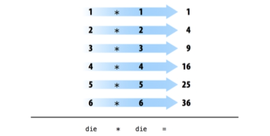
> die - 1 [1] 0 1 2 3 4 5 > die / 2 [1] 0.5 1.0 1.5 2.0 2.5 3.0 > die * die [1] 1 4 9 16 25 36 If you are a big fan of linear algebra (and who is not?), Then you probably noticed that R does not always follow the rules of matrix multiplication. Instead, R uses per-element multiplication. When you work with a set of numbers, R will apply a specific operation to each element in the set separately. For example, when we launch die - 1 , then R subtracts a unit from each element in die .
When using several vectors in operations, R first equalizes the lengths of the vectors and only then elementwise performs the operation itself. For example, when performing the operation die * die , R aligns the lengths of the two vectors, and then multiplies the first value from the first vector by the first value from the second vector, etc., until all the elements are multiplied. The result of this operation will be a new vector of the same length as the two multiplied vectors.
If you pass R two vectors of different lengths, then R will “repeat” / “loop” a vector of shorter length until it becomes equal in length to the larger vector. The change in the smaller vector is not a constant change (the source vector does not change), it is supplemented only for the duration of the operation. If the length of the larger vector is not a multiple of the length of the smaller vector, then R will issue a warning. This behavior is known as vector recycling and allows R to perform in-element operations:
> 1:4 [1] 1 2 3 4 > die [1] 1 2 3 4 5 6 > die + 1:2 [1] 2 4 4 6 6 8 > die + 1:4 [1] 2 4 6 8 6 8 Warning message: In die + 1:4 : longer object length is not a multiple of shorter object length By-element operations are extremely important in R, as they allow processing of groups of values in a specific order. When you begin to work with a variety of data, per-element operations will make sure that the data from one observation exactly matches the data from another observation. By-element operations also simplify the creation of eigenfunctions and programs on R.
However, do not think that R abandoned the traditional matrix work. You just need to use the right operator.
Use the % *% operator for the inner work, and % o% for the outer work.
> die %*% die [,1] [1,] 91 > die %o% die [,1] [,2] [,3] [,4] [,5] [,6] [1,] 1 2 3 4 5 6 [2,] 2 4 6 8 10 12 [3,] 3 6 9 12 15 18 [4,] 4 8 12 16 20 24 [5,] 5 10 15 20 25 30 [6,] 6 12 18 24 30 36 You can also transpose the matrix using the t function and calculate its determinant using the det function.
Do not worry if you are not familiar with these features. Their description is simply found in the documentation, besides, in this book you will not need them.
Now that you have figured out how to perform math operations on the values of the die, let's see how we can program the throw (throwing the dice). To throw the dice you need something more magical than basic arithmetic; You will need to randomly select one of the dice values. But for this you need a function .
Functions
R initially contains many useful and surprising functions that you can use for such tasks as, for example, generating a random sample. For example, you can round the number with the round () function, or calculate the factorial of the number with the factorial () function. Using functions is quite simple. You write the name of the function you want to use, and in parentheses the data over which you need to perform the calculations:
> round(3.1415) [1] 3 > factorial(3) [1] 6 The data you pass to a function is called a function argument. The argument can be as raw data, objects or other functions of R. In the latter case, R will perform functions in the order of decreasing their nesting.
> mean(1:6) [1] 3.5 > mean(die) [1] 3.5 > round(mean(die)) [1] 4 To our happiness, there is a function in R that can help us with the implementation of the die roll. You can simulate a die roll using the sample function. The sample function takes two arguments: the vector x and the name parameter size . The sample function returns the size of elements from the x vector.
> sample(x = 1:4, size = 2) [1] 2 1 To simulate a die roll and get one numeric value as a result, set x to die and highlight / select one random element.
Each time you start you will have a different value:
> sample(x = die, size = 1) [1] 2 > sample(x = die, size = 1) [1] 6 > sample(x = die, size = 1) [1] 1 The set of functions in R takes several arguments that help it perform its stated task. You can pass as many arguments to the function as long as each of them is separated by a comma.
You could have noticed that I assigned the values die and 1 to the specific named arguments of the sample function x and size . Each argument in the R function has its own name. You can specify which values to assign to which arguments, as was shown in the previous example. It becomes extremely convenient to do when you pass multiple parameters into one function; Named arguments eliminate errors with passing the wrong data to the wrong arguments. The use of names is the solution of each and is not mandatory. You may notice that R users often do not specify the name of the first argument of the function. The previous code can be rewritten as follows:
> sample(die, size = 1) [1] 2 > sample(die, 1) [1] 2 Very often, the name of the first argument is not very meaningful, and most often it is clear what data must be passed to the function first.
How do you know which argument names to use? If you try to use names that the function does not expect, you will most likely get an error message:
> round(3.1415, corners = 4) Error in round(3.1415, corners = 4) : unused argument (corners = 4) If you doubt which argument names can be passed to a function, you can use the args function, which will list all possible named arguments of a particular function. To do this, put the name of the function in parentheses as an argument - args (the name of the function) . For example, you see that the round function takes two arguments — one with the name x , the second with the name digits :
> args(round) function (x, digits = 0) NULL > args(sample) function (x, size, replace = FALSE, prob = NULL) NULL > args(args) function (name) NULL Did you notice that the digits name argument in the round function is set to 0 by default? Often functions in R accept optional parameters, such as digits . These arguments are considered optional because they have already been assigned a default value. You can pass a new value for such a parameter if you want, or use the default provided. For example, round rounds clean to the nearest 0 decimal values by default. To overwrite the default, pass in the new:
> round(3.14151617, digits = 3) [1] 3.142 You should specify named arguments after the first or second argument of the function when calling a function with multiple arguments. Why? First, it will help you and other developers understand the code. It is often clear what the transmitted data refers to in the first and second arguments. However, you will need a phenomenal memory to remember all subsequent argument names for all existing functions in R. Secondly, and more importantly, this will avoid annoying errors.
If you do not use named arguments, then R will automatically match the arguments with the parameters in the order in which you passed them. For example, in the example below, the first die value will be assigned to the variable x , the second value 1 will be assigned to size .
> sample(die, 1) [1] 2 The more arguments you pass, the greater the likelihood of diverging the order in which arguments are passed. As a result, values can be passed to the wrong arguments. Named arguments exclude such errors. R will always correctly assign a value to a named argument, regardless of the order in which they follow.
> sample(size = 1, x = die) [1] 4 Sampling with recovery
If you set size = 2, then you almost modeled the dice rolls. Before you run this code, think a minute, what’s wrong?
sample returns two numbers, one for each die:
> sample(size = 2, x = die) [1] 5 3 I said “almost” because this method works a bit differently than we expect. If we run the code above several times, we note that the second value will never coincide with the first, which means we will never be able to throw two triples or two sixes. What's happening?
By default, sample samples without recovery . To figure out what this means, imagine that sample places all die values in an urn (basket). Then sample randomly fetches the values one by one from the basket for building the sample. After sample has used the selected value, it is not returned back and cannot be reused. Therefore, if the value of 6 falls for the first time, then the second time it will no longer be able to drop; 6 is no longer in the basket.
A side effect of this behavior is the dependence of subsequent shots from previous ones. In the real world, however, when you roll a pair of dice, each dice is independent of the others. If 6 falls on the first die, this does not prevent the loss of 6 and on the second die. You can recreate this behavior in sample by simply passing the optional argument replace = TRUE .
> sample(die, size = 2, replace = TRUE) [1] 1 1 The argument replace = TRUE changes the operation of the sample function. Our initial basket example is a good way to show how a sample works with and without replacement / repair. sample with replacement after selecting an arbitrary value from the basket returns it back. As a result, we have achieved the desired effect.
Sampling with recovery is an easy way to create independent random samples (blah blah blah ...). Each value in your sample will be a sample of size 1 that does not depend on other values. The correct way to simulate a roll of a pair of dice:
> sample(die, size = 2, replace = TRUE) [1] 6 4 You can praise yourself; you have just implemented your first simulation on R! You now have a method to simulate a roll of a die. If you want to add the dropped dice values, you can simply pass the result of the sample to the sum function.
> dice <- sample(die, size = 2, replace = TRUE) > dice [1] 3 3 > sum(dice) [1] 6 What happens if you call dica several times? Will R generate a new pair of values for each roll? Let's try:
> dice [1] 3 3 > dice [1] 3 3 > dice [1] 3 3 Not. Each time you call dica in R, the values that were once stored in this object will be displayed as a result.
However, it would be logical to have an object that would be able to generate a new pair of values with each simulation of the throw. You can implement this by writing your own R function.
We write our own functions
Recall that you already have a working code on R that simulates a roll of two dice:
> die <- 1:6 > dice <- sample(die, size = 2, replace = T) > dice [1] 2 5 You can reprint this code into the console R each time you want to make a new dice roll. However, this is quite a strange way. It would be much more convenient to use this code once in our function and then call it. This we now do. We are going to write the roll function, which you can use to simulate a roll of a virtual dice. When you are done, the function will work as follows: each time roll () is called, R will return the sum of the values of the two rolled dice.
> roll() > 8 > roll() > 3 > roll() > 7 Functions may seem magical and bizarre, but they are nothing more than the type of object in R. Functions do not contain data, but code. This code is stored in a format that allows it to be reused in other programs.
Function constructor
Each function in R consists of three main parts: a name, a body, a list of arguments. To write your own function, you need to create these three parts and store them in an object using the function () function :
my_function <- function() {} function will create a function from any R code that you place between the opening and closing curly braces. For example, you can transfer all of your previous dice-throw code into a function:
> roll <- function() { + die <- 1:6 + dice <- sample(die, size = 2, replace =T) + sum(dice) + } After opening the curly bracket, the command line R will wait for the remaining commands to enter until it finds the closing curly bracket of the function.
Remember to save the result of the function function to an R object. This object will now become a function. To use the new function, enter the object name, opening and closing parentheses:
> roll() [1] 7 > roll() [1] 10 > roll() [1] 11 You can count the parentheses after the object name as a trigger that runs the code inside the object for execution. If you enter a function name without parentheses, then R will show you directly the code stored in the function object:
> roll function() { die <- 1:6 dice <- sample(die, size = 2, replace =T) sum(dice) } The code that you put into a function is called the function body . When a function is executed in R, R will execute all the code that is in the function body and return the value that will be calculated on the last line. If the last line does not return any value, it means that your function will not return anything.
Here is the code that displays the result after the execution on the last line:
> dice > 1 + 1 > sqrt(2) But the code that does not display the results after the execution on the last line:
> dice <- sample(die, size = 2, replace = TRUE) > two <- 1 + 1 > a <- sort(2) Notice the difference? These lines of code do not return a value to the command line; they store values in the object.
Arguments
What would happen if we removed one line from our code and renamed the die variable to bones :
> roll2 <- function() { + dice <- sample(bones, size=2, replace=T) + sum(dice) + } If you now call the roll2 function , you will get an error message. For the function to work correctly, a bones object is needed , but such an object does not exist:
> roll2() Error in sample(bones, size = 2, replace = T) : object 'bones' not found You can pass bones as an argument to the roll2 function . To do this, you must specify the name of the argument in parentheses in the function declaration:
> roll2 <- function(bones) { + dice <- sample(bones, size = 2, replace = TRUE) + sum(dice) + } Now the roll2 function will work if you pass bones to it . You can use this to throw away different types of dice.
Remember that we are throwing two dice:
> roll2(1:4) [1] 5 > roll2(1:6) [1] 8 > roll2(1:20) [1] 12 Note that when you call roll2, it will still return an error if you do not pass values to the bones argument .
> roll2() Error in sample(bones, size = 2, replace = TRUE) : argument "bones" is missing, with no default You can prevent this error from appearing on such a call by setting the default bones argument . You can do this as follows:
> roll2 <- function(bones = 1:6){ + dice <- sample(bones, size = 2, replace = TRUE) + sum(dice) + } Now you can safely call the roll2 function to simulate a roll of two dice:
> roll2() [1] 8 > roll2(1:100) [1] 82 You can pass an unlimited number of arguments to your functions. To do this, list their names separated by commas between parentheses when declaring a function. Each time the function is started, R will automatically replace the argument name with the value that was passed to it. If no value was passed, then R will use the default value.
Summing up, function is used to declare eigenfunctions in R. The function code is placed between two curly braces. Arguments are specified after the function name, separated by commas between two parentheses.
After you have written your function, R will perceive it as any other function. Just imagine how useful and convenient this is. Have you ever tried to create a new function for Excel and add it to the panel with the menu? Or a new type of animation as a new option in PowerPoint? When you work with a programming language, all this becomes available to you. While learning the R language, you will learn how to create new, customizable, reproducible tools for any occasion. In part 3, we take a closer look at the functions.
Remember:
Scripts
To be continued…
Source: https://habr.com/ru/post/268731/
All Articles