Ant optimization and network algorithms
As you can see, we have a lull here. But our creative search does not stop, and the first October publication will be devoted to ACO (Ant Colony Optimization)

Paying tribute to the author, we will not publish here the last part of the article containing an example in JavaScript, but we will suggest that you try it out on the original site. Under the cat, you will find a translation of the theoretical part, which tells about the intricacies of ant optimization in various scenarios.
The Ant Colony Algorithm (ACO) optimization was first proposed by Marco Dorigo in 1992. This optimization technique is based on the strategy that ants adhere to, paving the way for food. In addition, ACO is a special case of swarm intelligence. Swarm intelligence is a kind of artificial intelligence where decentralized collective behavior is used to solve problems. Ant algorithms are most widely used for combinatorial optimization, for example, when solving the traveling salesman problem, although they are also applicable as a variety of planning and routing solutions.
')
An important advantage of ant algorithms in comparison with other optimization algorithms is their inherent ability to adapt to dynamic environments. That is why they are so indispensable for network routing, where frequent changes are common, which have to adapt.
Ants in nature
In order to fully understand ACO, it is important to have a good understanding of the ant behavior in nature, which served as the basis for the algorithm.
When searching for food, ants follow a relatively simple set of rules. With all the simplicity, these rules allow ants to communicate and jointly optimize paths to prey. One of the main properties of all these rules is the use of pheromone traces. It is with the help of pheromones that some ants tell others where food is found and how to get to it. As a rule, if an ant stumbles on a pheromone trail, it can be calculated that it will find food by it. However, ants do not run on the first pheromone trail. Depending on its smelliness, an ant can go on a different path or even choose a random path where there is no pheromone. On average, the more the pheromone trail smells, the more likely it is that the ant decides to roll.
Over time, the pheromone trail gradually disappears if other ants do not update it. Thus, pheromone traces that do not lead to food, sooner or later are abandoned, and the ants have to create new routes to new food sources.
To understand how this process develops over time, and how a colony optimizes its own behavior, consider the following example:

This is the way the ant went to food. From our point of view, this path is clearly not optimal, although it is possible. But here the fun begins. Further, other ants from the same colony stumble upon the pheromone trail of the first. Most of them follow the original route, but some choose another, more direct route:

Although the first pheromone trail at this point may be more fragrant, the second trail begins to develop - corresponding to the path to which some ants accidentally fold. In this scenario, it is important that the second path is preferable, since the insects that chose it will reach the food and get it faster than the ants that followed the first path. For example, one ant can spend 3 minutes to run along the first path from the anthill to the food source and back, but another ant runs the other route twice as fast and, accordingly, has two pheromone traces there. For this reason, the short path soon becomes more fragrant than the first. Accordingly, the first trail is used less and less often, until finally it disappears, and only a new, shorter path remains.

It is for this reason that the most dense pheromone traces are usually deposited along the most advantageous routes, which gradually become preferable for all ants from this anthill.
In brief, we note that this is a simplified picture of the behavior of ants in nature; In addition, different types of ants use pheromones a little differently.
Algorithm
This article will discuss the use of the ACO algorithm to solve the traveling salesman problem. If you are not familiar with the essence of this task, we refer you to the article.
The main part of the ACO algorithm consists of only a few steps. First, each ant from the colony builds a solution based on the available pheromone traces. Next, the ants leave traces along the segments of the selected route, depending on the quality of the worked out solution. In the example with the task of a traveling salesman, these would be ribs (or sections of a path between cities). Finally, when all the ants have completed laying the route and pheromone traces, the pheromone begins to steadily evaporate at each segment. Then such a sequence of stages is repeatedly run until an adequate solution is obtained.
Solution Development
As mentioned above, when laying a route, an ant usually runs along the most fragrant pheromone trail. However, if the ant begins to consider other decisions, besides that which is currently considered optimal, then a fraction of randomness is introduced into the decision-making process. In addition, the heuristic value of the solutions is calculated and taken into account, due to which the search develops towards optimal options. In the example of the traveling salesman problem, the heuristic is usually related to the length of the rib to the next city to be reached. The shorter the edge, the more likely it is that the route will continue along it.
Consider how this is implemented mathematically:
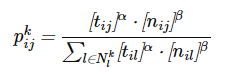
This equation calculates the probability of choosing a particular component of the solution. Here tij means the amount of pheromone in the interval between the states i and j, and nij - its heuristic value. α and β are the parameters by which the importance of the pheromone trace and heuristic information are controlled when a component is selected.
In the code, this information is usually expressed as a choice in the style of the roulette algorithm:
In the context of the traveling salesman problem, the state corresponds to a specific city in the graph. In our case, the ant will choose the next item depending on the distance that will have to be overcome, and on the amount of pheromone in this segment.
Local Pheromone Update
The process of local pheromone update is activated whenever an ant gets a successful solution. This step simulates the laying of pheromone traces left by ants in nature on the way to food. As you remember from the above, in nature, the most successful routes get the most pheromones, since they are overcome by ants faster. In ACO, this characteristic is reproduced as follows: the amount of pheromone on the segment of the path will vary depending on how successful a particular solution. If we take for example the task of a traveling salesman, the pheromone would be delayed on the roads between cities, depending on the total distance.

The diagram shows pheromone traces left on the segments between points (“cities”) in a typical traveling salesman problem.
Before we look at the implementation in code, let's turn to mathematics:

Here Ck is defined as the total cost of the solution; in the traveling salesman problem, this would be the total path length. Q is simply a parameter that helps to correct the amount of pheromone left, usually it is set to 1. We summarize Q / Ck for each solution that used component (i, j), then this value is taken as the amount of pheromone that will be left for component (i, j).
To clarify the situation, let's look at a simple example of this process as applied to the traveling salesman problem ...
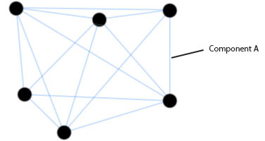
Here we have a typical graph from the traveling salesman problem and want to calculate how much pheromone should be on segment A. Suppose that three ants passed along this edge when laying routes. Also suppose that the total lengths of the three routes are as follows:
Tour 1: 450
Tour 2: 380
Tour 1: 460
To calculate how much pheromone should be on each of them, simply summarize:
Then we add this value to the pheromone value in the segment:
Now - a simple example with the code:
In this example, we simply iterate over the routes of the entire colony, extracting each route and applying a pheromone value to each edge of the route.
Global Pheromone Update
Global pheromone update is the stage at which the pheromone evaporates from the length of the path. This stage is applied after each iteration of the algorithm, when each ant has successfully built a route and applied the local update rule.
Global pheromone update is mathematically described as:
τij ← (1 − ρ) ⋅τij
where τij is a pheromone in the segment between the states i and j, and ρ is the parameter with which the rate of volatilization is corrected.
In the code, the situation can be represented as follows:
Optimization
The ACO algorithm allows for many optimization options, the most important of which are elitist and MaxMin. Depending on the task, these variations may well be more efficient than the standard ACO system discussed above. Fortunately, it will not be difficult for us to expand the algorithm so that it takes into account these two modifications.
Elite variety
In elite ACO systems, the most successful string of ants, as well as the most productive ant of all at the local update stage, leaves slightly more pheromone than all the others. Therefore, the colony adapts decisions made on the model of those who have the best history of achievements. If everything goes well, the quality of the search increases.
From a mathematical point of view, the elite local update procedure is almost the same as the usual one, with one small addition:

Where e is the parameter used to correct the additional volume of pheromone that is set aside at the best (or "elite") solution.
Maxmin
The MaxMin algorithm resembles the elite version of ACO in that it gives priority to "high rating" solutions. However, MaxMin does not just give additional weight to elite solutions, but permits to leave the pheromone trace only to the most efficient string, which corresponds to the best global solution. In addition, MaxMin requires that pheromone traces fall within a range between a certain minimum and maximum value. The algorithm is based on the idea that if the amount of pheromone on any particular track belongs to a certain range, then it will be possible to avoid a premature convergence on non-optimal solutions.
In many implementations of MaxMin, the ant that leaves pheromone traces is considered the most successful. Then this algorithm is modified in such a way that the ability to leave a trace is preserved only in the “globally” best ant. This process stimulates such a search, which is initially distributed throughout the available space, but subsequently focuses on optimal routes, allowing for perhaps minimal corrections.
Finally, the minimum and maximum values can either be passed as parameters, or adaptively set in code.
An interesting practical solution to TSP in JavaScript - on the author's website
Paying tribute to the author, we will not publish here the last part of the article containing an example in JavaScript, but we will suggest that you try it out on the original site. Under the cat, you will find a translation of the theoretical part, which tells about the intricacies of ant optimization in various scenarios.
The Ant Colony Algorithm (ACO) optimization was first proposed by Marco Dorigo in 1992. This optimization technique is based on the strategy that ants adhere to, paving the way for food. In addition, ACO is a special case of swarm intelligence. Swarm intelligence is a kind of artificial intelligence where decentralized collective behavior is used to solve problems. Ant algorithms are most widely used for combinatorial optimization, for example, when solving the traveling salesman problem, although they are also applicable as a variety of planning and routing solutions.
')
An important advantage of ant algorithms in comparison with other optimization algorithms is their inherent ability to adapt to dynamic environments. That is why they are so indispensable for network routing, where frequent changes are common, which have to adapt.
Ants in nature
In order to fully understand ACO, it is important to have a good understanding of the ant behavior in nature, which served as the basis for the algorithm.
When searching for food, ants follow a relatively simple set of rules. With all the simplicity, these rules allow ants to communicate and jointly optimize paths to prey. One of the main properties of all these rules is the use of pheromone traces. It is with the help of pheromones that some ants tell others where food is found and how to get to it. As a rule, if an ant stumbles on a pheromone trail, it can be calculated that it will find food by it. However, ants do not run on the first pheromone trail. Depending on its smelliness, an ant can go on a different path or even choose a random path where there is no pheromone. On average, the more the pheromone trail smells, the more likely it is that the ant decides to roll.
Over time, the pheromone trail gradually disappears if other ants do not update it. Thus, pheromone traces that do not lead to food, sooner or later are abandoned, and the ants have to create new routes to new food sources.
To understand how this process develops over time, and how a colony optimizes its own behavior, consider the following example:
This is the way the ant went to food. From our point of view, this path is clearly not optimal, although it is possible. But here the fun begins. Further, other ants from the same colony stumble upon the pheromone trail of the first. Most of them follow the original route, but some choose another, more direct route:
Although the first pheromone trail at this point may be more fragrant, the second trail begins to develop - corresponding to the path to which some ants accidentally fold. In this scenario, it is important that the second path is preferable, since the insects that chose it will reach the food and get it faster than the ants that followed the first path. For example, one ant can spend 3 minutes to run along the first path from the anthill to the food source and back, but another ant runs the other route twice as fast and, accordingly, has two pheromone traces there. For this reason, the short path soon becomes more fragrant than the first. Accordingly, the first trail is used less and less often, until finally it disappears, and only a new, shorter path remains.
It is for this reason that the most dense pheromone traces are usually deposited along the most advantageous routes, which gradually become preferable for all ants from this anthill.
In brief, we note that this is a simplified picture of the behavior of ants in nature; In addition, different types of ants use pheromones a little differently.
Algorithm
This article will discuss the use of the ACO algorithm to solve the traveling salesman problem. If you are not familiar with the essence of this task, we refer you to the article.
The main part of the ACO algorithm consists of only a few steps. First, each ant from the colony builds a solution based on the available pheromone traces. Next, the ants leave traces along the segments of the selected route, depending on the quality of the worked out solution. In the example with the task of a traveling salesman, these would be ribs (or sections of a path between cities). Finally, when all the ants have completed laying the route and pheromone traces, the pheromone begins to steadily evaporate at each segment. Then such a sequence of stages is repeatedly run until an adequate solution is obtained.
Solution Development
As mentioned above, when laying a route, an ant usually runs along the most fragrant pheromone trail. However, if the ant begins to consider other decisions, besides that which is currently considered optimal, then a fraction of randomness is introduced into the decision-making process. In addition, the heuristic value of the solutions is calculated and taken into account, due to which the search develops towards optimal options. In the example of the traveling salesman problem, the heuristic is usually related to the length of the rib to the next city to be reached. The shorter the edge, the more likely it is that the route will continue along it.
Consider how this is implemented mathematically:
This equation calculates the probability of choosing a particular component of the solution. Here tij means the amount of pheromone in the interval between the states i and j, and nij - its heuristic value. α and β are the parameters by which the importance of the pheromone trace and heuristic information are controlled when a component is selected.
In the code, this information is usually expressed as a choice in the style of the roulette algorithm:
rouletteWheel = 0 states = ant.getUnvisitedStates() for newState in states do rouletteWheel += Math.pow(getPheromone(state, newState), getParam('alpha')) * Math.pow(calcHeuristicValue(state, newState), getParam('beta')) end for randomValue = random() wheelPosition = 0 for newState in states do wheelPosition += Math.pow(getPheromone(state, newState), getParam('alpha')) * Math.pow(calcHeuristicValue(state, newState), getParam('beta')) if wheelPosition >= randomValue do return newState end for In the context of the traveling salesman problem, the state corresponds to a specific city in the graph. In our case, the ant will choose the next item depending on the distance that will have to be overcome, and on the amount of pheromone in this segment.
Local Pheromone Update
The process of local pheromone update is activated whenever an ant gets a successful solution. This step simulates the laying of pheromone traces left by ants in nature on the way to food. As you remember from the above, in nature, the most successful routes get the most pheromones, since they are overcome by ants faster. In ACO, this characteristic is reproduced as follows: the amount of pheromone on the segment of the path will vary depending on how successful a particular solution. If we take for example the task of a traveling salesman, the pheromone would be delayed on the roads between cities, depending on the total distance.
The diagram shows pheromone traces left on the segments between points (“cities”) in a typical traveling salesman problem.
Before we look at the implementation in code, let's turn to mathematics:
Here Ck is defined as the total cost of the solution; in the traveling salesman problem, this would be the total path length. Q is simply a parameter that helps to correct the amount of pheromone left, usually it is set to 1. We summarize Q / Ck for each solution that used component (i, j), then this value is taken as the amount of pheromone that will be left for component (i, j).
To clarify the situation, let's look at a simple example of this process as applied to the traveling salesman problem ...
Here we have a typical graph from the traveling salesman problem and want to calculate how much pheromone should be on segment A. Suppose that three ants passed along this edge when laying routes. Also suppose that the total lengths of the three routes are as follows:
Tour 1: 450
Tour 2: 380
Tour 1: 460
To calculate how much pheromone should be on each of them, simply summarize:
componentNewPheromone = (Q / 450) + (Q / 380) + (Q / 460)
Then we add this value to the pheromone value in the segment:
componentPheromone = componentPheromone + componentNewPheromone
Now - a simple example with the code:
for ant in colony do tour = ant.getTour(); pheromoneToAdd = getParam('Q') / tour.distance(); for cityIndex in tour do if lastCity(cityIndex) do edge = getEdge(cityIndex, 0) else do edge = getEdge(cityIndex, cityIndex+1) end if currentPheromone = edge.getPheromone(); edge.setPheromone(currentPheromone + pheromoneToAdd) end for end for In this example, we simply iterate over the routes of the entire colony, extracting each route and applying a pheromone value to each edge of the route.
Global Pheromone Update
Global pheromone update is the stage at which the pheromone evaporates from the length of the path. This stage is applied after each iteration of the algorithm, when each ant has successfully built a route and applied the local update rule.
Global pheromone update is mathematically described as:
τij ← (1 − ρ) ⋅τij
where τij is a pheromone in the segment between the states i and j, and ρ is the parameter with which the rate of volatilization is corrected.
In the code, the situation can be represented as follows:
for edge in edges updatedPheromone = (1 - getParam('rho')) * edge.getPheromone() edge.setPheromone(updatedPheromone) end for Optimization
The ACO algorithm allows for many optimization options, the most important of which are elitist and MaxMin. Depending on the task, these variations may well be more efficient than the standard ACO system discussed above. Fortunately, it will not be difficult for us to expand the algorithm so that it takes into account these two modifications.
Elite variety
In elite ACO systems, the most successful string of ants, as well as the most productive ant of all at the local update stage, leaves slightly more pheromone than all the others. Therefore, the colony adapts decisions made on the model of those who have the best history of achievements. If everything goes well, the quality of the search increases.
From a mathematical point of view, the elite local update procedure is almost the same as the usual one, with one small addition:
Where e is the parameter used to correct the additional volume of pheromone that is set aside at the best (or "elite") solution.
Maxmin
The MaxMin algorithm resembles the elite version of ACO in that it gives priority to "high rating" solutions. However, MaxMin does not just give additional weight to elite solutions, but permits to leave the pheromone trace only to the most efficient string, which corresponds to the best global solution. In addition, MaxMin requires that pheromone traces fall within a range between a certain minimum and maximum value. The algorithm is based on the idea that if the amount of pheromone on any particular track belongs to a certain range, then it will be possible to avoid a premature convergence on non-optimal solutions.
In many implementations of MaxMin, the ant that leaves pheromone traces is considered the most successful. Then this algorithm is modified in such a way that the ability to leave a trace is preserved only in the “globally” best ant. This process stimulates such a search, which is initially distributed throughout the available space, but subsequently focuses on optimal routes, allowing for perhaps minimal corrections.
Finally, the minimum and maximum values can either be passed as parameters, or adaptively set in code.
An interesting practical solution to TSP in JavaScript - on the author's website
Source: https://habr.com/ru/post/268513/
All Articles