Phase portraits "on the fingers" or what can be found out about diffraction solutions without solving it
Very often in a number of sciences there is a situation when the model of the process under consideration is reduced to a differential equation. Moreover, in most real-world problems this equation is rather difficult to solve, or completely impossible. And here in the full voice of the eternal question: what to do?
Meet: phase portraits (they are also phase diagrams). In simple terms, the phase portrait is how the values describing the state of the system (aka dynamic variables) depend on each other. In the case of mechanical movement, this is the coordinate and speed, in electricity it is charge and current, in a known population problem this is the number of predators and prey, etc.
What are good phase portraits? And the fact that they can be constructed without solving the dynamic equations of the system. In some cases, building a phase portrait becomes a very simple task. However, at the same time, phase portraits give the thoughtful observer a lot of information about the behavior of the system.
Let's start with a simple example - small oscillations (also called harmonic). Small fluctuations are found in almost every sphere of the natural sciences. For definiteness, we will consider oscillations of a metal rod suspended at one of the ends (a special case of the so-called physical pendulum). It can be shown that its oscillations are described by the following differential equation:
')
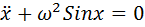
Where x is the angle of deflection of the rod from the vertical, a point above x means the time derivative, and the coefficient in front of the sine depends on the size and mass of the rod.
If the amplitude (range) of the oscillations is small enough, the sine can be approximately replaced by its argument (do you remember the first remarkable limit, no?). In this case, the equation takes the following form:

This equation is easily solved by regular methods, but let's try to apply the phase portraits method to it. To do this, multiply the equation by the derivative and integrate it once in time:
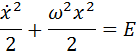
It turned out the expression, the first member of which looks like kinetic energy. This is not accidental - in fact, we received precisely the law of conservation of energy. The constant E on the right-hand side (the total energy of the system per unit mass) can take different values, which correspond to different initial states of the system.
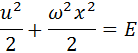
We introduce the notation:

The conservation law we obtained turned into a curve equation on the (x, u) plane:
For different values of E, we get different curves. Let's draw several such lines for different values of energy:

The horizontal axis represents the value of x , the vertical axis - u
Each of the obtained lines is called a phase trajectory. When the state of the system changes, the point that represents it moves along one of these paths, the arrows indicate the direction of movement of the image point.
The graph shows that the values of speed and coordinates vary cyclically, that is, periodically repeated. From this we can conclude that the system described by the equation considered will oscillate. Bingo! This is how the pendulum behaves, and if the equation is solved, the solution will have the form of periodic functions (namely, combinations of sine and cosine).
However, it should be remembered that replacing the sine with its argument is justified only for small deviations (from 10 degrees and less), so we cannot trust those trajectories that go beyond the boundaries of the area bounded by bold dashed lines, that is, of the four trajectories only orange Reliably displays reality. In addition, since x is an angle, its values corresponding to 180 and -180 degrees describe the same position of the rod, that is, the right and left dotted lines (thin) on the graph are in fact the same line.
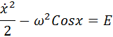
Now, since we understand the essence, we can move on to something more complicated. Above, we greatly simplified the equation and, at the same time, limited ourselves to small oscillations. A mathematician would say that we linearized the equation and neglected non-linear effects. So let's include nonlinearity in consideration. Let's return to the very first equation - with a sine. If we repeat with him what we did with the linear equation, we get the following conservation law:
Depending on the energy value, we again get different curves, which are shown in the following figure, with the same energy values as in the first diagram, and the same colors for the lines.
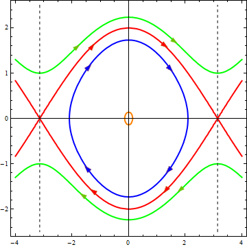
The horizontal axis represents the value of x , the vertical axis - u
As you can see, the processes occurring in the system have become more diverse:
At low energies (orange and blue trajectories), an oscillatory mode exists, but the oscillations are no longer harmonic — the phase trajectories are no longer in the shape of ellipses.
At high energies (green trajectory), the oscillations no longer exist; instead, we get a rotational motion with variable speed. And indeed, if the “rod” is sufficiently “pushed”, it will rotate, slowing down when lifting and accelerating during descent.
At a certain intermediate value of energy, a special set of trajectories is obtained, which separate the regions corresponding to different types of motion from each other and are therefore called separatrices . And yes, the energy value for the red curve was chosen by me in such a way that in the nonlinear case a separatrix would turn out. Each separatrix branch is a trajectory corresponding to a particular type of movement. Let's look at the diagram: the movement starts at a very small speed from one extreme position of the rod, as it approaches the equilibrium position, the speed increases, and after that the imaging point slows down more and more to the extreme position, where it stops. This corresponds to the fact that we raise the rod vertically up and release it, zipping through the equilibrium position, it rises to the top point on the other side and stops.
And now let's see how close to the truth our conclusions are based on phase portraits. Here is a graph of solving a linear equation:
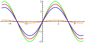
Time is plotted on the horizontal axis, x is on the vertical axis
... and non-linear:
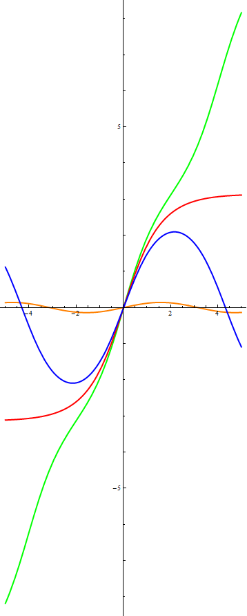
Time is plotted on the horizontal axis, x is on the vertical axis
The color markings on these graphs are the same as on the phase portraits. To judge how the correct conclusions were made on the basis of phase portraits, I give you, dear readers. I draw your attention to only one moment - oscillations in a linear case occur synchronously - with the same frequency. In the non-linear case, the oscillation frequency with a larger amplitude (blue line) turns out to be less than that of a vibration with a small amplitude (orange line). This is another confirmation that non-linear oscillations are not harmonic.
And finally: this is just a superficial excursion into the method of phase portraits, and the phrase "on the fingers" fell into the title for a reason. Those who decide to go deep into the vicissitudes of this subject will see that much more lies behind the phase portraits.
Meet: phase portraits (they are also phase diagrams). In simple terms, the phase portrait is how the values describing the state of the system (aka dynamic variables) depend on each other. In the case of mechanical movement, this is the coordinate and speed, in electricity it is charge and current, in a known population problem this is the number of predators and prey, etc.
What are good phase portraits? And the fact that they can be constructed without solving the dynamic equations of the system. In some cases, building a phase portrait becomes a very simple task. However, at the same time, phase portraits give the thoughtful observer a lot of information about the behavior of the system.
Let's start with a simple example - small oscillations (also called harmonic). Small fluctuations are found in almost every sphere of the natural sciences. For definiteness, we will consider oscillations of a metal rod suspended at one of the ends (a special case of the so-called physical pendulum). It can be shown that its oscillations are described by the following differential equation:
')
Where x is the angle of deflection of the rod from the vertical, a point above x means the time derivative, and the coefficient in front of the sine depends on the size and mass of the rod.
If the amplitude (range) of the oscillations is small enough, the sine can be approximately replaced by its argument (do you remember the first remarkable limit, no?). In this case, the equation takes the following form:
This equation is easily solved by regular methods, but let's try to apply the phase portraits method to it. To do this, multiply the equation by the derivative and integrate it once in time:
It turned out the expression, the first member of which looks like kinetic energy. This is not accidental - in fact, we received precisely the law of conservation of energy. The constant E on the right-hand side (the total energy of the system per unit mass) can take different values, which correspond to different initial states of the system.
We introduce the notation:
The conservation law we obtained turned into a curve equation on the (x, u) plane:
For different values of E, we get different curves. Let's draw several such lines for different values of energy:
The horizontal axis represents the value of x , the vertical axis - u
Each of the obtained lines is called a phase trajectory. When the state of the system changes, the point that represents it moves along one of these paths, the arrows indicate the direction of movement of the image point.
The graph shows that the values of speed and coordinates vary cyclically, that is, periodically repeated. From this we can conclude that the system described by the equation considered will oscillate. Bingo! This is how the pendulum behaves, and if the equation is solved, the solution will have the form of periodic functions (namely, combinations of sine and cosine).
However, it should be remembered that replacing the sine with its argument is justified only for small deviations (from 10 degrees and less), so we cannot trust those trajectories that go beyond the boundaries of the area bounded by bold dashed lines, that is, of the four trajectories only orange Reliably displays reality. In addition, since x is an angle, its values corresponding to 180 and -180 degrees describe the same position of the rod, that is, the right and left dotted lines (thin) on the graph are in fact the same line.
Now, since we understand the essence, we can move on to something more complicated. Above, we greatly simplified the equation and, at the same time, limited ourselves to small oscillations. A mathematician would say that we linearized the equation and neglected non-linear effects. So let's include nonlinearity in consideration. Let's return to the very first equation - with a sine. If we repeat with him what we did with the linear equation, we get the following conservation law:
Depending on the energy value, we again get different curves, which are shown in the following figure, with the same energy values as in the first diagram, and the same colors for the lines.
The horizontal axis represents the value of x , the vertical axis - u
As you can see, the processes occurring in the system have become more diverse:
At low energies (orange and blue trajectories), an oscillatory mode exists, but the oscillations are no longer harmonic — the phase trajectories are no longer in the shape of ellipses.
At high energies (green trajectory), the oscillations no longer exist; instead, we get a rotational motion with variable speed. And indeed, if the “rod” is sufficiently “pushed”, it will rotate, slowing down when lifting and accelerating during descent.
At a certain intermediate value of energy, a special set of trajectories is obtained, which separate the regions corresponding to different types of motion from each other and are therefore called separatrices . And yes, the energy value for the red curve was chosen by me in such a way that in the nonlinear case a separatrix would turn out. Each separatrix branch is a trajectory corresponding to a particular type of movement. Let's look at the diagram: the movement starts at a very small speed from one extreme position of the rod, as it approaches the equilibrium position, the speed increases, and after that the imaging point slows down more and more to the extreme position, where it stops. This corresponds to the fact that we raise the rod vertically up and release it, zipping through the equilibrium position, it rises to the top point on the other side and stops.
And now let's see how close to the truth our conclusions are based on phase portraits. Here is a graph of solving a linear equation:
Time is plotted on the horizontal axis, x is on the vertical axis
... and non-linear:
Time is plotted on the horizontal axis, x is on the vertical axis
The color markings on these graphs are the same as on the phase portraits. To judge how the correct conclusions were made on the basis of phase portraits, I give you, dear readers. I draw your attention to only one moment - oscillations in a linear case occur synchronously - with the same frequency. In the non-linear case, the oscillation frequency with a larger amplitude (blue line) turns out to be less than that of a vibration with a small amplitude (orange line). This is another confirmation that non-linear oscillations are not harmonic.
And finally: this is just a superficial excursion into the method of phase portraits, and the phrase "on the fingers" fell into the title for a reason. Those who decide to go deep into the vicissitudes of this subject will see that much more lies behind the phase portraits.
Source: https://habr.com/ru/post/268507/
All Articles