Blocks. The internal structure of the Caché database file. Part 2
This publication is a continuation of my article , in which I described how the Caché database is designed from the inside. In it, I described the types of blocks, how they are related, and how they relate to the global. That article had a theory. I created a project that allows you to visualize the tree of blocks - and in this article you will see all this. Welcome under cat.
To demonstrate, I created a new database and cleared all globals that Caché initializes by default for the newly created database. Create a simple global:
')
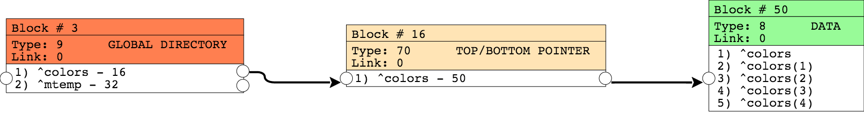
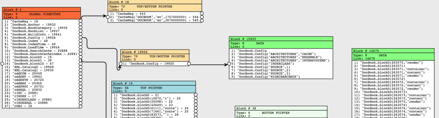
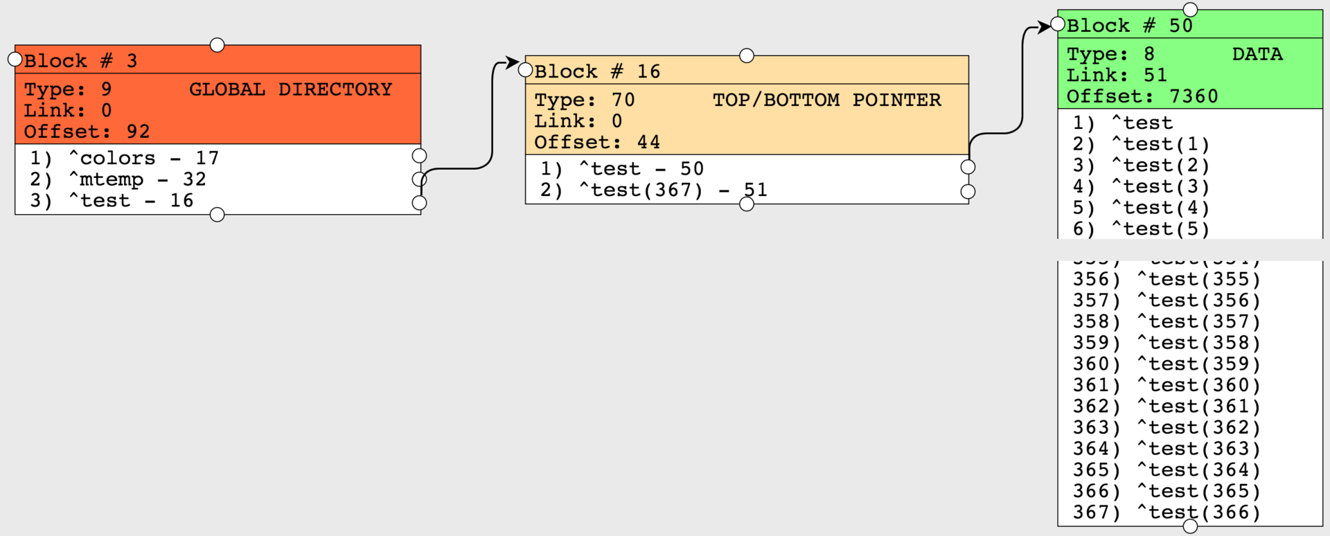
Pay attention to the picture illustrating the blocks of the created global. The global is simple, so we, of course, see its description in a block of type 9 (block of the catalog of globals). Then the “upper and lower pointer” block (type 70) goes right away, since the global tree is still shallow, and you can immediately point to the link to the data block that still fits into one 8KB block.
Now we write to another global value in such a quantity that they could not fit in one block anymore - and we will see how new nodes appear in the block of pointers, which will refer to new data blocks that did not fit in the first block.
We will write down 50 values with a length of 1000 characters. Recall that the block size of our database is 8192 bytes.
Pay attention to the following picture:
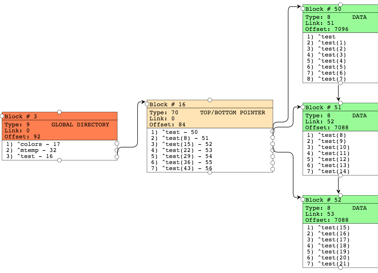
At the block pointer level, we now have several nodes that reference data blocks. Each data block has links to the next block (“right link”). Offset - indicates the number of bytes used in this block of data.
Now we will try to model block splitting. We add to the first block so many values that the total block size of 8KB is exceeded, which will result in this block being split into two.
The result can be seen below:

Block 50 was split, it was supplemented with new data, and the values that were pushed out of it are now in block 58. The link to this block appeared in the block of pointers. Other blocks have not changed.
When writing lines longer than 8KB (data block size) we get “long data” blocks. We can simulate such a situation, for example, by writing lines of 10,000 bytes in size.
Let's look at the result:

As a result, the structure of the blocks in the picture is preserved, because we did not add new nodes of the global, but only changed the values. But the Offset value (the number of bytes occupied) for all blocks has changed. For example, for block No. 51, the new value of Offset was 172, against 7088 the previous time. It is clear that now, when the new value cannot fit in the block, the pointer to the last data byte should have changed, but where are our data now stored? At the moment, my project has not yet implemented the ability to display information about "big blocks". Let's turn to the ^ REPAIR utility to display information about the new content of block No. 51.
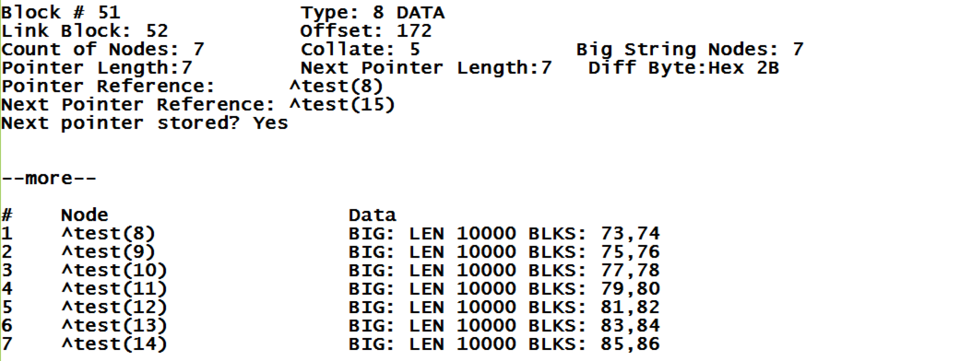
I will dwell in more detail on what this utility shows us. We see a link to the right block number 52, the same number was specified in the parent block of pointers at the next node. Global sorting is type 5. The number of nodes with large lines is 7. In some cases, a block may contain both data values for some nodes, and long lines for others, all within one block. We also see which global link should be expected at the beginning of the next block (Next Pointer Reference).
About blocks of long lines: here we see that the keyword BIG is specified as the value for the global, which tells us that the data is actually in “large blocks”. Further on the same line we see the total length of the contained line, and the list of blocks that store this value. We can try to look at the "block of long lines", at number 73.
Unfortunately, this block is output unencrypted. But here we can notice that after the overhead information from the block header (which is always 28 bytes long), the data entered is used. And knowing what data, it is easy to decipher what is indicated in the title:
Let me remind you that the data in block 51 occupy only 172 bytes. It happened at the moment when we kept great values. It turns out that the block has become almost empty - the payload is 172 bytes, and it takes 8kb! It is clear that in such a situation, the free space will eventually be filled with new values, but also Caché gives us the opportunity to compress such a global one. To do this, the % Library.GlobalEdit class has a CompactGlobal method. In order to make sure that this method is effective, we will repeat our example, but with a large amount of data, for example, having created 500 nodes.
Execute the CompactGlobal method:
Let's look at the result. The block of pointers we now have only 2 nodes, i.e. our values all went into two data blocks, whereas earlier we had 72 nodes in a pointer block. Thus, we got rid of 70 blocks, reducing, thus, the time to access the data with a full crawl of the global, as less reads are required on the blocks.
CompactGlobal accepts several parameters for input, such as the name of the global, the database and the percentage of filling that we want to receive, with a default value of 90. And now we see that Offset (the number of bytes used) became equal to 7360, which is approximately the most 90% filling. Several parameters of the output function: how many megabytes are processed and the number of megabytes after compression. Previously, globals were compressed using the ^ GCOMPACT utility, which is currently considered obsolete.
It is worth noting that the situation in which the blocks may remain incompletely filled is quite normal. Moreover, global compression may not always be desirable. For example, if your global is more readable and practically does not change, then compression can help. But if the global is actively changing, then a certain sparsity in the data blocks will help to split the blocks less often, and the recording of new data will occur faster.
In the next part I will talk about another possibility of my project, which was implemented in the framework of the recently passed hackathon at InterSystems school - about the distribution map of base blocks and its practical application.
To demonstrate, I created a new database and cleared all globals that Caché initializes by default for the newly created database. Create a simple global:
set ^colors(1)="red" set ^colors(2)="blue" set ^colors(3)="green" set ^colors(4)="yellow" ')
Pay attention to the picture illustrating the blocks of the created global. The global is simple, so we, of course, see its description in a block of type 9 (block of the catalog of globals). Then the “upper and lower pointer” block (type 70) goes right away, since the global tree is still shallow, and you can immediately point to the link to the data block that still fits into one 8KB block.
Now we write to another global value in such a quantity that they could not fit in one block anymore - and we will see how new nodes appear in the block of pointers, which will refer to new data blocks that did not fit in the first block.
We will write down 50 values with a length of 1000 characters. Recall that the block size of our database is 8192 bytes.
set str="" for i=1:1:1000 { set str=str_"1" } for i=1:1:50 { set ^test(i)=str } quit Pay attention to the following picture:
At the block pointer level, we now have several nodes that reference data blocks. Each data block has links to the next block (“right link”). Offset - indicates the number of bytes used in this block of data.
Now we will try to model block splitting. We add to the first block so many values that the total block size of 8KB is exceeded, which will result in this block being split into two.
Code example
set str="" for i=1:1:1000 { set str=str_"1" } set ^test(3,1)=str set ^test(3,2)=str set ^test(3,3)=str The result can be seen below:
Block 50 was split, it was supplemented with new data, and the values that were pushed out of it are now in block 58. The link to this block appeared in the block of pointers. Other blocks have not changed.
Example with long lines
When writing lines longer than 8KB (data block size) we get “long data” blocks. We can simulate such a situation, for example, by writing lines of 10,000 bytes in size.
Code example
set str="" for i=1:1:10000 { set str=str_"1" } for i=1:1:50 { set ^test(i)=str } Let's look at the result:
As a result, the structure of the blocks in the picture is preserved, because we did not add new nodes of the global, but only changed the values. But the Offset value (the number of bytes occupied) for all blocks has changed. For example, for block No. 51, the new value of Offset was 172, against 7088 the previous time. It is clear that now, when the new value cannot fit in the block, the pointer to the last data byte should have changed, but where are our data now stored? At the moment, my project has not yet implemented the ability to display information about "big blocks". Let's turn to the ^ REPAIR utility to display information about the new content of block No. 51.
I will dwell in more detail on what this utility shows us. We see a link to the right block number 52, the same number was specified in the parent block of pointers at the next node. Global sorting is type 5. The number of nodes with large lines is 7. In some cases, a block may contain both data values for some nodes, and long lines for others, all within one block. We also see which global link should be expected at the beginning of the next block (Next Pointer Reference).
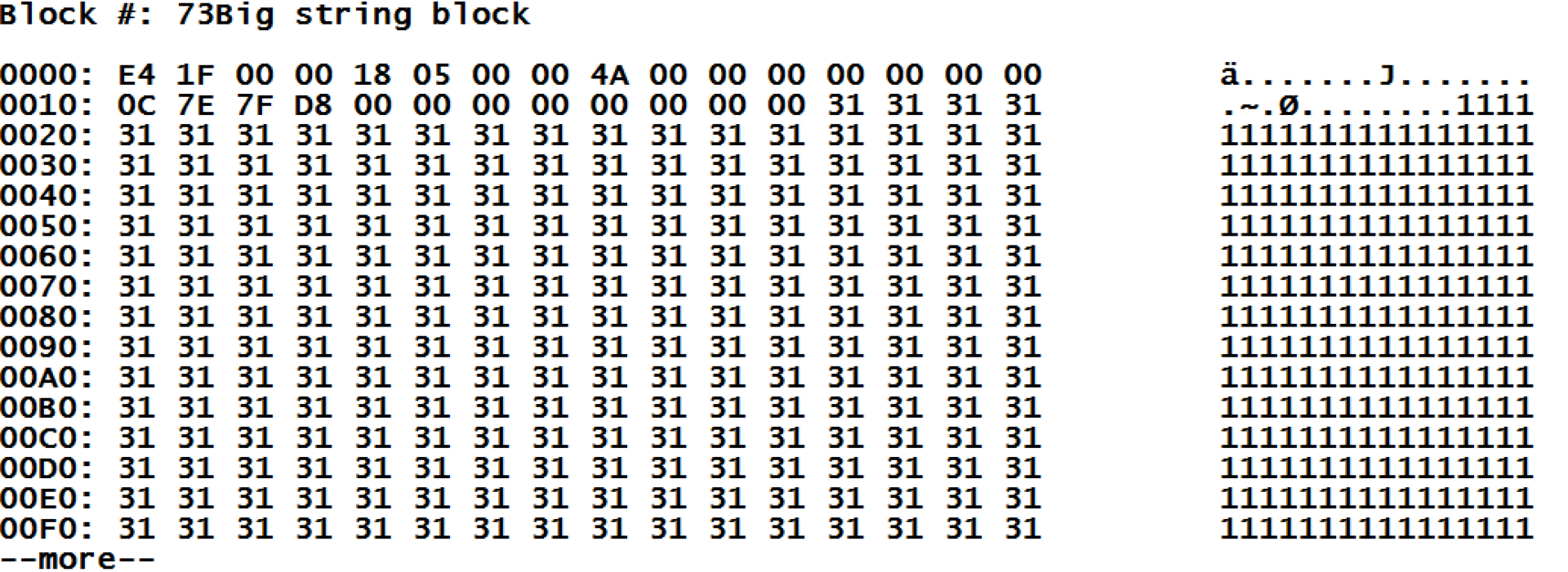
About blocks of long lines: here we see that the keyword BIG is specified as the value for the global, which tells us that the data is actually in “large blocks”. Further on the same line we see the total length of the contained line, and the list of blocks that store this value. We can try to look at the "block of long lines", at number 73.
Unfortunately, this block is output unencrypted. But here we can notice that after the overhead information from the block header (which is always 28 bytes long), the data entered is used. And knowing what data, it is easy to decipher what is indicated in the title:
| Position | Value | Description | Read more |
| 0-3 | E4 1F 00 00 | offset indicates end of data | it turns out 8164 plus 28 bytes of the header is 8192 bytes, unit is full. |
| four | 18 | block type | the value 24, as we remember , is the type for a block of large strings. |
| five | 05 | sorting | Sort 5, this is "standard caché" |
| 8-11 | 4A 00 00 00 | right connection | it turned out 74, as we remember our value is stored in block 73 and 74 |
Let me remind you that the data in block 51 occupy only 172 bytes. It happened at the moment when we kept great values. It turns out that the block has become almost empty - the payload is 172 bytes, and it takes 8kb! It is clear that in such a situation, the free space will eventually be filled with new values, but also Caché gives us the opportunity to compress such a global one. To do this, the % Library.GlobalEdit class has a CompactGlobal method. In order to make sure that this method is effective, we will repeat our example, but with a large amount of data, for example, having created 500 nodes.
That's what we did.
Below we have shown not all the blocks, but the meaning should be clear. We have a lot of data blocks, but with a small number of nodes.
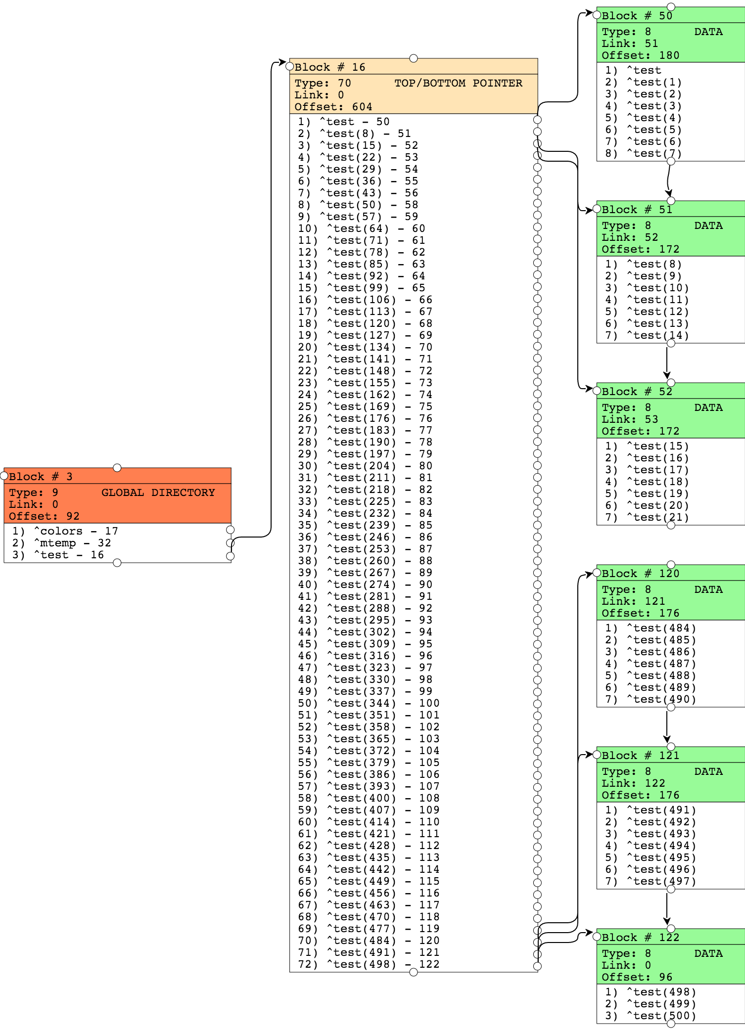
kill ^test for l=1000,10000 { set str="" for i=1:1:l { set str=str_"1" } for i=1:1:500 { set ^test(i)=str } } quit Below we have shown not all the blocks, but the meaning should be clear. We have a lot of data blocks, but with a small number of nodes.
Execute the CompactGlobal method:
w ##class(%GlobalEdit).CompactGlobal("test","c:\intersystems\ensemble\mgr\habr") Let's look at the result. The block of pointers we now have only 2 nodes, i.e. our values all went into two data blocks, whereas earlier we had 72 nodes in a pointer block. Thus, we got rid of 70 blocks, reducing, thus, the time to access the data with a full crawl of the global, as less reads are required on the blocks.
CompactGlobal accepts several parameters for input, such as the name of the global, the database and the percentage of filling that we want to receive, with a default value of 90. And now we see that Offset (the number of bytes used) became equal to 7360, which is approximately the most 90% filling. Several parameters of the output function: how many megabytes are processed and the number of megabytes after compression. Previously, globals were compressed using the ^ GCOMPACT utility, which is currently considered obsolete.
It is worth noting that the situation in which the blocks may remain incompletely filled is quite normal. Moreover, global compression may not always be desirable. For example, if your global is more readable and practically does not change, then compression can help. But if the global is actively changing, then a certain sparsity in the data blocks will help to split the blocks less often, and the recording of new data will occur faster.
In the next part I will talk about another possibility of my project, which was implemented in the framework of the recently passed hackathon at InterSystems school - about the distribution map of base blocks and its practical application.
Source: https://habr.com/ru/post/268195/
All Articles