The continuation of the candy problem (or, once again, the Central Limit Theorem)
Recently, viktorpanasiuk published a task about sweets that “hooked” on many (in particular, koldyr published his analytical solution on Habré), including me. The practical task, from the pastry engineer, was formulated as follows: “To find the maximum permissible deviation of the candy mass during its production, so that the net of a box consisting of n = 12 pieces of them does not exceed M = 310 ± 7 grams in 90% of cases. The distribution law is considered normal. "
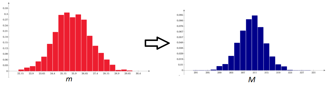
The author solved the problem, based on the assumption of a normal distribution of candies by weight, and found the average candy mass (obviously, equal to µ = M / n = 25.83 g) and the standard deviation σ = 1.23 g. Using the Monte Carlo method, i.e. the generation of N * n random numbers with a Gaussian distribution of candies with mean µ and standard deviation σ confirms the correctness of the solution. The mass distribution of the boxes is Gaussian, and its parameters are close to those found analytically (calculations in Mathcad Express in the MCDX and XPS formats are attached ). The left graph shows the histogram of the distribution density (by mass) of candies, and the right graph shows the distribution of the boxes, respectively.
')
In the final article cited, the author mentions a slightly modified (in practice, more relevant) problem of determining the boundaries of the mass of an individual candy, beyond which this (too large or small) candy must be discarded so that the boxes meet the initial conditions (310 ± 7 g in 90 % of cases). In my opinion, the original article already contains a solution, you just have to look at it from a slightly different point of view.
To take the final step in the reasoning, let us recall once again the central limit theorem (CLT), which can be interpreted as (see, for example, Wikipedia ) that the sum of n independent identically distributed random variables (with the same or approximately the same mean and variance) has the distribution close to normal. Note: in the condition of the theorem there are no assumptions about the nature of the distribution of the initial random variables! Statistics of sweets, therefore, can be any , and their numbers in the box n = 12, as experience shows, is enough to talk about normalization of the total weight.
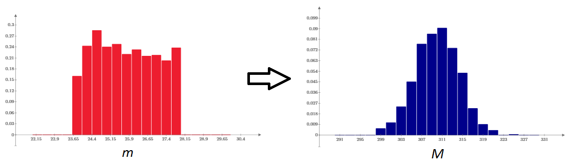
Let's, in order to make sure that the weight of the box is normalized, we choose a model of uniform distribution of individual candies by weight. Adding 12 independent pseudo-random numbers and repeating this computational experiment N times, make sure that the histogram of the distribution density of the candy boxes is well described by the normal law (the graph on the right), while the distribution of each of the 12 candies is, in fact, uniform (left graph) :
If you choose the limits of rejection of too large and too small candies so that the standard deviation of the mass of candies is the same σ = 1.23 g, then, according to the CLT, the dispersion of the box (the sum of n = 12 candies) will be the desired value of σ 2 * n.
This is the desired algorithm. Suppose we have a candy machine that is adjusted to an average candy mass µ. Next, we can, controlling the sample value of the candy dispersion, narrow the allowable interval beyond which the candy is rejected. Regardless of the nature of the distribution, the choice of such an interval, which will provide the standard deviation of the candy mass σ = 1.23, will solve the problem (due to the normalization of the box weight, due to the CLT).
The author solved the problem, based on the assumption of a normal distribution of candies by weight, and found the average candy mass (obviously, equal to µ = M / n = 25.83 g) and the standard deviation σ = 1.23 g. Using the Monte Carlo method, i.e. the generation of N * n random numbers with a Gaussian distribution of candies with mean µ and standard deviation σ confirms the correctness of the solution. The mass distribution of the boxes is Gaussian, and its parameters are close to those found analytically (calculations in Mathcad Express in the MCDX and XPS formats are attached ). The left graph shows the histogram of the distribution density (by mass) of candies, and the right graph shows the distribution of the boxes, respectively.
')
In the final article cited, the author mentions a slightly modified (in practice, more relevant) problem of determining the boundaries of the mass of an individual candy, beyond which this (too large or small) candy must be discarded so that the boxes meet the initial conditions (310 ± 7 g in 90 % of cases). In my opinion, the original article already contains a solution, you just have to look at it from a slightly different point of view.
To take the final step in the reasoning, let us recall once again the central limit theorem (CLT), which can be interpreted as (see, for example, Wikipedia ) that the sum of n independent identically distributed random variables (with the same or approximately the same mean and variance) has the distribution close to normal. Note: in the condition of the theorem there are no assumptions about the nature of the distribution of the initial random variables! Statistics of sweets, therefore, can be any , and their numbers in the box n = 12, as experience shows, is enough to talk about normalization of the total weight.
Let's, in order to make sure that the weight of the box is normalized, we choose a model of uniform distribution of individual candies by weight. Adding 12 independent pseudo-random numbers and repeating this computational experiment N times, make sure that the histogram of the distribution density of the candy boxes is well described by the normal law (the graph on the right), while the distribution of each of the 12 candies is, in fact, uniform (left graph) :
If you choose the limits of rejection of too large and too small candies so that the standard deviation of the mass of candies is the same σ = 1.23 g, then, according to the CLT, the dispersion of the box (the sum of n = 12 candies) will be the desired value of σ 2 * n.
This is the desired algorithm. Suppose we have a candy machine that is adjusted to an average candy mass µ. Next, we can, controlling the sample value of the candy dispersion, narrow the allowable interval beyond which the candy is rejected. Regardless of the nature of the distribution, the choice of such an interval, which will provide the standard deviation of the candy mass σ = 1.23, will solve the problem (due to the normalization of the box weight, due to the CLT).
Source: https://habr.com/ru/post/267939/
All Articles