Greenplum db
We continue a series of articles on technologies used in the work of the data warehouse (Data Warehouse, DWH) of our bank. In this article I will try to briefly and a little superficially talk about Greenplum - a DBMS based on postgreSQL, which is the core of our DWH. The article will not provide installation logs, configs, etc. - and without this, the note turned out to be quite voluminous. Instead, I will talk about the general DBMS architecture, methods for storing and filling data, backups, and also list several problems we encountered during operation.

A little bit about our installations:
')
For how it works, please under the cat!
So, Greenplum (GP) is a relational DBMS that has massive parallel processing without Shared Nothing. For a detailed understanding of how GP works, you need to define basic terms:
Master instance (also known as “master”) - Postgres instance, which is both a coordinator and an entry point for users in a cluster;
Master host ("server master") - the server on which the Master instance is running;
Secondary master instance - Postgres instance, which is a backup master, is included in the work in case the main master is unavailable (switching occurs manually);
Primary segment instance ("segment") - Postgres instance, which is one of the segments. It is the segments that directly store data, perform operations with them, and give the results to the master (in general). In fact, a segment is the most common PostgreSQL 8.2.15 instance with configured WAL replication to its mirror on another server:
Mirror segment instance (“mirror”) - the Postgres instance, which is a mirror of one of the primary segments, automatically assumes the role of primary in the event of a fall:
GP supports only 1-to-1 segment replication: for each primary there can be only one mirror.
Segment host ("server-segment") - a server that runs one or more segments and / or mirrors.
In general, a GP cluster consists of several server segments, a single master server, and a single master server, interconnected by one or several fast (10g, infiniband) networks, usually interconnect:

Fig. 1. The composition of the cluster and the network interaction of elements. Here - green and red lines - separate interconnect networks, blue line - external, client network.
The use of several interconnect-networks allows, firstly, to increase the capacity of the channel of interaction between the segments between themselves, and secondly, to ensure the fault tolerance of the cluster (in the event of a failure of one of the networks, all traffic is redistributed among the remaining ones).
When choosing the number of server segments, it is important to choose the cluster ratio “number of processors / TB of data” depending on the planned load profile on the database - the more processor cores are in the data unit, the faster the cluster will perform “heavy” operations, and also work with compressed tables.
When choosing the number of segments in a cluster (which is generally not tied to the number of servers), remember the following:
The Greenplum implements the classic data sharding scheme. Each table is N + 1 tables on all segments of the cluster, where N is the number of segments (+1 in this case is the table on the master, there is no data in it). Each segment contains 1 / N rows of the table. The logic of partitioning a table into segments is defined by a distribution key (field), a field on the basis of which data any line can be assigned to one of the segments.
The key (field or set of fields) of distribution is a very important concept in GP. As mentioned above, Greenplum operates at the speed of the slowest segment, which means that any bias in the amount of data (both within one table and across the entire database) between segments leads to degradation of cluster performance, as well as other problems. That is why one should carefully select the field for distribution - the distribution of the number of occurrences of values in it should be as even as possible. Whether you have chosen the distribution key correctly will be prompted by the service field gp_segment_id, which exists in each table - it contains the number of the segment on which the specific row is stored.
An important caveat: GP does not support UPDATE fields over which the table is distributed.
In both cases, we distributed the table across the num_field field. In the first case, we inserted 20 unique values into this field, and, as you can see, the GP laid out all the lines into different segments. In the second case, 20 identical values were inserted in the field, and all lines were placed on one segment.
In case the table does not have suitable fields for use as a distribution key, you can use random distribution (DISTRIBUTED RANDOMLY). The field for distribution can be changed in an already created table, but after that it must be redistributed.
It is through the distribution field that Greenplum performs the most optimal JOINs: if the fields for which the JOIN is made are distribution keys in both tables, the JOIN is executed locally on the segment. If this condition is not true, GP will have to either redistribute both tables to the desired field, or throw one of the tables entirely on each segment (operation BROADCAST) and then then join the tables locally on the segments.
As you can see, in the second case, two additional steps appear in the query plan (one for each of the tables participating in the query): Redistribute Motion . In fact, before executing the request, GP redistributes both tables into segments using the logic of the num_field_2 field, and not the initial distribution key, the num_field field.
In general, all client interaction with the cluster is conducted only through the master — it is he who responds to clients, gives them the result of the query, etc. Regular client users do not have network access to segment servers.
To speed up the loading of data into the cluster, bulk load is used - parallel loading of data from / to the client simultaneously from several segments. Bulk load is only possible from clients with access to interconnects. Usually such clients are ETL servers and other systems that need to download a large amount of data (in Figure 1 they are designated as ETL / Pro client ).
For parallel data loading into segments, the gpfdist utility is used. In fact, the utility raises a web server on a remote server that provides access via the gpfdist and http protocols to the specified folder:
After launch, the directory and all files in it become accessible to the usual wget. For example, let's create a file in the directory served by gpfdist and treat it as a regular table.
Also, but with a slightly different syntax, external web tables are created. Their peculiarity is that they refer to the http protocol and can work with data provided by third-party web servers (apache, etc.).
Separately, it is possible to create external tables for data lying on a distributed Hadoop filesystem (hdfs) - a separate gphdfs component is responsible for this in GP. To ensure its operation on each server that is part of a GP cluster, it is necessary to install the Hadoop libraries and assign a path to them in one of the system database variables. Creating an external table that accesses data in hdfs will look something like this:
Here hadoop_name_node is the address of the hostnames, /tmp/test_file.csv is the path to the desired file on hdfs.
When referring to such a table, Greenplum finds out at Hadoop's NEAMNODs the location of the necessary data blocks on datas, which are then accessed from segment servers in parallel. Naturally, all the nodes of the Hadoop cluster must be in the interconnect networks of the Greenplum cluster. Such a scheme of work allows to achieve a significant increase in speed, even compared with gpfdist. Interestingly, the logic of selecting segments for reading data from danod hdfs is very nontrivial. For example, the GP can start to pull data from all the data points with only two segment servers, and with a repeated similar request, the interaction scheme may change.
There is also a type of external tables that refer to files on a segment server or a file on a master, as well as the result of executing a command on a segment server or on a master. By the way, the good old COPY from has not gone away and can also be used, but compared to what was described above, it works more slowly.
As mentioned earlier, the GP cluster uses full wizard redundancy using the replication mechanism of transactional logs controlled by a special agent (gpsyncagent). In this case, automatic switching of the master role to the backup instance is not supported. To switch to the backup master you need:
As you can see, switching is not difficult at all and can be automated when taking certain risks.
The reservation scheme of the segments is similar to that for the master, the differences are quite small. If one of the segments fails (the postgres instance stops responding to the master during the timeout), the segment is marked as failed and its mirror is automatically launched instead (in fact, absolutely similar to the postgres instance). Replication of the segment data in its mirror is based on WAL (Wright Ahead Log).
It is worth noting that a rather important place in the planning process of the GP cluster architecture is the location of the segment mirrors on the servers, since the GP gives complete freedom in choosing the locations of the segments and their mirrors: using a special segment map, they can be placed on different servers different directories and make use of different ports. Consider two boundary options:

Option 1: all mirrors of segments located on host N are on host N + 1
In this case, if one of the servers on the server-neighbor fails, it turns out to be twice the number of running segments. As mentioned above, the cluster performance is equal to the performance of the slowest segment, and therefore, in the event of a single server failure, the performance of the database is at least halved.
However, such a scheme also has positive aspects: when working with a failed server, only one server becomes the weak point of the cluster - the same one where the segments have moved.
Option 2: all the mirrors of the segments located on the host N are uniformly “smeared” on the servers N + 1, N + 2 ... N + M, where M is the number of segments on the server
In this case, in the event of a server failure, the increased load is evenly distributed among several servers, not much affecting the overall performance of the cluster. However, the risk of failure of the entire cluster is significantly increased - it is enough to fail one of the M servers adjacent to the failed one initially.
The truth, as often happens, is somewhere in the middle - you can arrange several mirrors of segments of one server on several other servers, you can combine servers into fault tolerance groups, and so on. The optimal configuration of the mirrors should be selected on the basis of specific cluster hardware data, idle severity, and so on.
Also in the mechanism of redundancy segments there is another nuance that affects the performance of the cluster. In case of failure of a mirror of one of the segments, the latter goes into change tracking mode — the segment logs all changes so that, when recovering the fallen mirror, apply them to it, and get a fresh, consistent copy of the data. In other words, when a mirror falls, the load created on the server’s disk subsystem by a segment without a mirror increases significantly.
When eliminating the cause of a segment failure (hardware problems, expired storage space, etc.), it must be returned to work manually using the special utility gprecoverseg (DBMS downtime is not required). In fact, this utility will copy the WA logs accumulated on the segment onto the mirror and pick up the fallen segment / mirror. If we are talking about the primary segment, initially it will be included in the work as a mirror for its mirror, which has become primary (the mirror and the main segment will work by exchanging roles). In order to bring everything back to normal, it will require a rebalance procedure - changing roles. Such a procedure also does not require downtime of the DBMS, but for the time of rebalance all sessions in the database are suspended.
If the damage of a fallen segment is so serious that simply copying data from WA-logs is not enough, it is possible to use a full recovery of a fallen segment - in this case, the postgresql instance will be created anew, but due to the fact that the restoration will be not incremental, the recovery process may take a long time.
Evaluating the performance of the Greenplum cluster is a rather loose concept. I decided to start with the tests performed in this article: habrahabr.ru/post/253017 , since the systems under consideration are in many ways similar. Since the cluster under test is significantly (8 times only by the number of servers) more powerful than the one given in the article above, we will take 10 times more test data. If you would like to see the results of other cases in this article, write in the comments, if possible I will try to test.
Initial data: a cluster of 24 segment servers, each server - 192 GB of memory, 40 cores. Number of primary segments in a cluster: 96.
So, in the first example, we create a table with 4 fields + a primary key for one of the fields. Then we fill the table with data (10,000,000 rows) and try a simple SELECT with several conditions. I remind you that the entire test is taken from the Postgres-XL article.
As you can see, the query execution time was 175 ms. Now let's try an example with a join on the distribution key of one table and on the usual field of another table.
4.6 . – .
, , , (, , ). , « / », .1. , .
Greenplum , . :
, , 20-30 .
, . , GP. , postgresql ( vacuum', WAL-) .
Greenplum — . , enterprise-level Data Warehouse ( — GP). postgresql Greenplum Data Warehouse DB.
, , — 17 2015 Pivotal , Greenplum open source , Big Data Product Suite .
UPD 28.10.2015. github: github.com/greenplum-db/gpdb
« »: 12 Dell EMC , Pivotal.
9.
A little bit about our installations:
')
- the project lives with us a little more than two years;
- 4 circuits from 10 to 26 cars;
- database size is about 30 TB;
- in the database about 10,000 tables;
- up to 700 queries per second.
For how it works, please under the cat!
1. General Architecture
So, Greenplum (GP) is a relational DBMS that has massive parallel processing without Shared Nothing. For a detailed understanding of how GP works, you need to define basic terms:
Master instance (also known as “master”) - Postgres instance, which is both a coordinator and an entry point for users in a cluster;
Master host ("server master") - the server on which the Master instance is running;
Secondary master instance - Postgres instance, which is a backup master, is included in the work in case the main master is unavailable (switching occurs manually);
Primary segment instance ("segment") - Postgres instance, which is one of the segments. It is the segments that directly store data, perform operations with them, and give the results to the master (in general). In fact, a segment is the most common PostgreSQL 8.2.15 instance with configured WAL replication to its mirror on another server:
/app/greenplum/greenplum-db-4.3.5.2/bin/postgres -D /data1/primary/gpseg76 -p 50004 -b 126 -z 96 --silent-mode=true -i -M quiescent -C 76 Mirror segment instance (“mirror”) - the Postgres instance, which is a mirror of one of the primary segments, automatically assumes the role of primary in the event of a fall:
/app/greenplum/greenplum-db-4.3.5.2/bin/postgres -D /data1/mirror/gpseg76 -p 51004 -b 186 -z 96 --silent-mode=true -i -M quiescent -C 76 GP supports only 1-to-1 segment replication: for each primary there can be only one mirror.
Segment host ("server-segment") - a server that runs one or more segments and / or mirrors.
In general, a GP cluster consists of several server segments, a single master server, and a single master server, interconnected by one or several fast (10g, infiniband) networks, usually interconnect:
Fig. 1. The composition of the cluster and the network interaction of elements. Here - green and red lines - separate interconnect networks, blue line - external, client network.
The use of several interconnect-networks allows, firstly, to increase the capacity of the channel of interaction between the segments between themselves, and secondly, to ensure the fault tolerance of the cluster (in the event of a failure of one of the networks, all traffic is redistributed among the remaining ones).
When choosing the number of server segments, it is important to choose the cluster ratio “number of processors / TB of data” depending on the planned load profile on the database - the more processor cores are in the data unit, the faster the cluster will perform “heavy” operations, and also work with compressed tables.
When choosing the number of segments in a cluster (which is generally not tied to the number of servers), remember the following:
- all server resources are divided between all segments on the server (the load of mirrors, if they are located on the same servers, can be conditionally ignored);
- each request on one segment cannot consume processor resources more than one CPU core. This means, for example, that if a cluster consists of 32-core servers with 4 GP segments onboard and is used on average to handle 3-4 simultaneous heavy, well-utilized CPU requests, the “hospital average” CPU will not recycle optimally. In this situation, it is better to increase the number of segments on the server to 6-8;
- The regular backup and restaraunt data process “out of the box” works only on clusters that have the same number of segments. It will be impossible to restore data stored on a cluster of 96 segments into a cluster of 100 segments without a file.
2. Data storage
The Greenplum implements the classic data sharding scheme. Each table is N + 1 tables on all segments of the cluster, where N is the number of segments (+1 in this case is the table on the master, there is no data in it). Each segment contains 1 / N rows of the table. The logic of partitioning a table into segments is defined by a distribution key (field), a field on the basis of which data any line can be assigned to one of the segments.
The key (field or set of fields) of distribution is a very important concept in GP. As mentioned above, Greenplum operates at the speed of the slowest segment, which means that any bias in the amount of data (both within one table and across the entire database) between segments leads to degradation of cluster performance, as well as other problems. That is why one should carefully select the field for distribution - the distribution of the number of occurrences of values in it should be as even as possible. Whether you have chosen the distribution key correctly will be prompted by the service field gp_segment_id, which exists in each table - it contains the number of the segment on which the specific row is stored.
An important caveat: GP does not support UPDATE fields over which the table is distributed.
Consider example 1 (hereinafter in the examples the cluster consists of 96 segments)
db=# create table distrib_test_table as select generate_series(1,20) as num_field distributed by (num_field); SELECT 20 db=# select count(1),gp_segment_id from distrib_test_table group by gp_segment_id order by gp_segment_id; count | gp_segment_id -------+--------------- 1 | 4 1 | 6 1 | 15 1 | 21 1 | 23 1 | 25 1 | 31 1 | 40 1 | 42 1 | 48 1 | 50 1 | 52 1 | 65 1 | 67 1 | 73 1 | 75 1 | 77 1 | 90 1 | 92 1 | 94 db=# truncate table distrib_test_table; TRUNCATE TABLE db=# insert into distrib_test_table values (1), (1), (1), (1), (1), (1), (1), (1), (1), (1), (1), (1), (1), (1), (1), (1), (1), (1), (1), (1); INSERT 0 20 db=# select count(1),gp_segment_id from distrib_test_table group by gp_segment_id order by gp_segment_id; count | gp_segment_id -------+--------------- 20 | 42 In both cases, we distributed the table across the num_field field. In the first case, we inserted 20 unique values into this field, and, as you can see, the GP laid out all the lines into different segments. In the second case, 20 identical values were inserted in the field, and all lines were placed on one segment.
In case the table does not have suitable fields for use as a distribution key, you can use random distribution (DISTRIBUTED RANDOMLY). The field for distribution can be changed in an already created table, but after that it must be redistributed.
It is through the distribution field that Greenplum performs the most optimal JOINs: if the fields for which the JOIN is made are distribution keys in both tables, the JOIN is executed locally on the segment. If this condition is not true, GP will have to either redistribute both tables to the desired field, or throw one of the tables entirely on each segment (operation BROADCAST) and then then join the tables locally on the segments.
Example 2: Joyne by distribution key
db=# create table distrib_test_table as select generate_series(1,192) as num_field, generate_series(1,192) as num_field_2 distributed by (num_field); SELECT 192 db=# create table distrib_test_table_2 as select generate_series(1,1000) as num_field, generate_series(1,1000) as num_field_2 distributed by (num_field); SELECT 1000 db=# explain select * from distrib_test_table sq db-# left join distrib_test_table_2 sq2 db-# on sq.num_field = sq2.num_field; QUERY PLAN ------------------------------------------------------------------------------------------ Gather Motion 96:1 (slice1; segments: 96) (cost=20.37..42.90 rows=861 width=16) -> Hash Left Join (cost=20.37..42.90 rows=9 width=16) Hash Cond: sq.num_field = sq2.num_field -> Seq Scan on distrib_test_table sq (cost=0.00..9.61 rows=9 width=8) -> Hash (cost=9.61..9.61 rows=9 width=8) -> Seq Scan on distrib_test_table_2 sq2 (cost=0.00..9.61 rows=9 width=8) Joyne is not a distribution key
db_dev=# explain select * from distrib_test_table sq left join distrib_test_table_2 sq2 on sq.num_field_2 = sq2.num_field_2; QUERY PLAN -------------------------------------------------------------------------------------------------------- Gather Motion 96:1 (slice3; segments: 96) (cost=37.59..77.34 rows=861 width=16) -> Hash Left Join (cost=37.59..77.34 rows=9 width=16) Hash Cond: sq.num_field_2 = sq2.num_field_2 -> Redistribute Motion 96:96 (slice1; segments: 96) (cost=0.00..26.83 rows=9 width=8) Hash Key: sq.num_field_2 -> Seq Scan on distrib_test_table sq (cost=0.00..9.61 rows=9 width=8) -> Hash (cost=26.83..26.83 rows=9 width=8) -> Redistribute Motion 96:96 (slice2; segments: 96) (cost=0.00..26.83 rows=9 width=8) Hash Key: sq2.num_field_2 -> Seq Scan on distrib_test_table_2 sq2 (cost=0.00..9.61 rows=9 width=8) As you can see, in the second case, two additional steps appear in the query plan (one for each of the tables participating in the query): Redistribute Motion . In fact, before executing the request, GP redistributes both tables into segments using the logic of the num_field_2 field, and not the initial distribution key, the num_field field.
3. Customer interaction
In general, all client interaction with the cluster is conducted only through the master — it is he who responds to clients, gives them the result of the query, etc. Regular client users do not have network access to segment servers.
To speed up the loading of data into the cluster, bulk load is used - parallel loading of data from / to the client simultaneously from several segments. Bulk load is only possible from clients with access to interconnects. Usually such clients are ETL servers and other systems that need to download a large amount of data (in Figure 1 they are designated as ETL / Pro client ).
For parallel data loading into segments, the gpfdist utility is used. In fact, the utility raises a web server on a remote server that provides access via the gpfdist and http protocols to the specified folder:
/usr/local/greenplum-loaders-4.3.0.0-build-2/bin/gpfdist -d /tmp/work/gpfdist_home -p 8081 -l /tmp/work/gpfdist_home/gpfdist8081.log After launch, the directory and all files in it become accessible to the usual wget. For example, let's create a file in the directory served by gpfdist and treat it as a regular table.
Example 3: gpfdist work
# ETL-: bash# for i in {1..1000}; do echo "$i,$(cat /dev/urandom | tr -dc 'a-zA-Z0-9' | fold -w 8 | head -n 1)"; done > /tmp/work/gpfdist_home/test_table.csv # # Greenplum DB: db=# create external table ext_test_table db-# (id integer, rand varchar(8)) db-# location ('gpfdist://etl_hostname:8081/test_table.csv') db-# format 'TEXT' (delimiter ',' NULL ' '); CREATE EXTERNAL TABLE db_dev=# select * from ext_test_table limit 100; NOTICE: External scan from gpfdist(s) server will utilize 64 out of 96 segment databases id | rand -----+---------- 1 | UWlonJHO 2 | HTyJNA41 3 | CBP1QSn1 4 | 0K9y51a3 … Also, but with a slightly different syntax, external web tables are created. Their peculiarity is that they refer to the http protocol and can work with data provided by third-party web servers (apache, etc.).
Separately, it is possible to create external tables for data lying on a distributed Hadoop filesystem (hdfs) - a separate gphdfs component is responsible for this in GP. To ensure its operation on each server that is part of a GP cluster, it is necessary to install the Hadoop libraries and assign a path to them in one of the system database variables. Creating an external table that accesses data in hdfs will look something like this:
db=# create external table hdfs_test_table db=# (id int, rand text) db=# location('gphdfs://hadoop_name_node:8020/tmp/test_file.csv') db=# format 'TEXT' (delimiter ','); Here hadoop_name_node is the address of the hostnames, /tmp/test_file.csv is the path to the desired file on hdfs.
When referring to such a table, Greenplum finds out at Hadoop's NEAMNODs the location of the necessary data blocks on datas, which are then accessed from segment servers in parallel. Naturally, all the nodes of the Hadoop cluster must be in the interconnect networks of the Greenplum cluster. Such a scheme of work allows to achieve a significant increase in speed, even compared with gpfdist. Interestingly, the logic of selecting segments for reading data from danod hdfs is very nontrivial. For example, the GP can start to pull data from all the data points with only two segment servers, and with a repeated similar request, the interaction scheme may change.
There is also a type of external tables that refer to files on a segment server or a file on a master, as well as the result of executing a command on a segment server or on a master. By the way, the good old COPY from has not gone away and can also be used, but compared to what was described above, it works more slowly.
4. Reliability and redundancy
4.1. Master Backup
As mentioned earlier, the GP cluster uses full wizard redundancy using the replication mechanism of transactional logs controlled by a special agent (gpsyncagent). In this case, automatic switching of the master role to the backup instance is not supported. To switch to the backup master you need:
- make sure that the master master is stopped (the process is killed and the postmaster.pid file is missing in the working directory of the master instance)
- on the backup wizard server, run the gpactivatestandby -d / master_instance_directory command
- switch the virtual ip-address to the server of the new wizard (there is no virtual ip mechanism in Greenplum, you need to use third-party tools).
As you can see, switching is not difficult at all and can be automated when taking certain risks.
4.2. Segment reservations
The reservation scheme of the segments is similar to that for the master, the differences are quite small. If one of the segments fails (the postgres instance stops responding to the master during the timeout), the segment is marked as failed and its mirror is automatically launched instead (in fact, absolutely similar to the postgres instance). Replication of the segment data in its mirror is based on WAL (Wright Ahead Log).
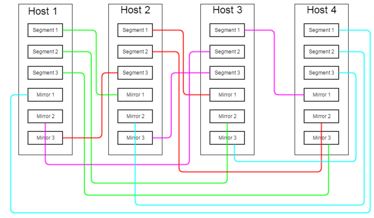
It is worth noting that a rather important place in the planning process of the GP cluster architecture is the location of the segment mirrors on the servers, since the GP gives complete freedom in choosing the locations of the segments and their mirrors: using a special segment map, they can be placed on different servers different directories and make use of different ports. Consider two boundary options:
Option 1: all mirrors of segments located on host N are on host N + 1
In this case, if one of the servers on the server-neighbor fails, it turns out to be twice the number of running segments. As mentioned above, the cluster performance is equal to the performance of the slowest segment, and therefore, in the event of a single server failure, the performance of the database is at least halved.
However, such a scheme also has positive aspects: when working with a failed server, only one server becomes the weak point of the cluster - the same one where the segments have moved.
Option 2: all the mirrors of the segments located on the host N are uniformly “smeared” on the servers N + 1, N + 2 ... N + M, where M is the number of segments on the server
In this case, in the event of a server failure, the increased load is evenly distributed among several servers, not much affecting the overall performance of the cluster. However, the risk of failure of the entire cluster is significantly increased - it is enough to fail one of the M servers adjacent to the failed one initially.
The truth, as often happens, is somewhere in the middle - you can arrange several mirrors of segments of one server on several other servers, you can combine servers into fault tolerance groups, and so on. The optimal configuration of the mirrors should be selected on the basis of specific cluster hardware data, idle severity, and so on.
Also in the mechanism of redundancy segments there is another nuance that affects the performance of the cluster. In case of failure of a mirror of one of the segments, the latter goes into change tracking mode — the segment logs all changes so that, when recovering the fallen mirror, apply them to it, and get a fresh, consistent copy of the data. In other words, when a mirror falls, the load created on the server’s disk subsystem by a segment without a mirror increases significantly.
When eliminating the cause of a segment failure (hardware problems, expired storage space, etc.), it must be returned to work manually using the special utility gprecoverseg (DBMS downtime is not required). In fact, this utility will copy the WA logs accumulated on the segment onto the mirror and pick up the fallen segment / mirror. If we are talking about the primary segment, initially it will be included in the work as a mirror for its mirror, which has become primary (the mirror and the main segment will work by exchanging roles). In order to bring everything back to normal, it will require a rebalance procedure - changing roles. Such a procedure also does not require downtime of the DBMS, but for the time of rebalance all sessions in the database are suspended.
If the damage of a fallen segment is so serious that simply copying data from WA-logs is not enough, it is possible to use a full recovery of a fallen segment - in this case, the postgresql instance will be created anew, but due to the fact that the restoration will be not incremental, the recovery process may take a long time.
5. Performance
Evaluating the performance of the Greenplum cluster is a rather loose concept. I decided to start with the tests performed in this article: habrahabr.ru/post/253017 , since the systems under consideration are in many ways similar. Since the cluster under test is significantly (8 times only by the number of servers) more powerful than the one given in the article above, we will take 10 times more test data. If you would like to see the results of other cases in this article, write in the comments, if possible I will try to test.
Initial data: a cluster of 24 segment servers, each server - 192 GB of memory, 40 cores. Number of primary segments in a cluster: 96.
So, in the first example, we create a table with 4 fields + a primary key for one of the fields. Then we fill the table with data (10,000,000 rows) and try a simple SELECT with several conditions. I remind you that the entire test is taken from the Postgres-XL article.
Test 1: SELECT with conditions
db=# CREATE TABLE test3 db-# (id bigint NOT NULL, db(# profile bigint NOT NULL, db(# status integer NOT NULL, db(# switch_date timestamp without time zone NOT NULL, db(# CONSTRAINT test3_id_pkey PRIMARY KEY (id) ) db-# distributed by (id); NOTICE: CREATE TABLE / PRIMARY KEY will create implicit index "test3_pkey" for table "test3" CREATE TABLE db=# insert into test3 (id , profile,status, switch_date) select a, round(random()*100000), round(random()*4), now() - '1 year'::interval * round(random() * 40) from generate_series(1,10000000) a; INSERT 0 10000000 db=# explain analyze select profile, count(status) from test3 db=# where status<>2 db=# and switch_date between '1970-01-01' and '2015-01-01' group by profile; Gather Motion 96:1 (slice2; segments: 96) (cost=2092.80..2092.93 rows=10 width=16) Rows out: 100001 rows at destination with 141 ms to first row, 169 ms to end, start offset by 0.778 ms. -> HashAggregate (cost=2092.80..2092.93 rows=1 width=16) Group By: test3.profile Rows out: Avg 1041.7 rows x 96 workers. Max 1061 rows (seg20) with 141 ms to end, start offset by 2.281 ms. Executor memory: 4233K bytes avg, 4233K bytes max (seg0). -> Redistribute Motion 96:96 (slice1; segments: 96) (cost=2092.45..2092.65 rows=1 width=16) Hash Key: test3.profile Rows out: Avg 53770.2 rows x 96 workers at destination. Max 54896 rows (seg20) with 71 ms to first row, 117 ms to end, start offset by 5.205 ms. -> HashAggregate (cost=2092.45..2092.45 rows=1 width=16) Group By: test3.profile Rows out: Avg 53770.2 rows x 96 workers. Max 54020 rows (seg69) with 71 ms to first row, 90 ms to end, start offset by 7.014 ms. Executor memory: 7882K bytes avg, 7882K bytes max (seg0). -> Seq Scan on test3 (cost=0.00..2087.04 rows=12 width=12) Filter: status <> 2 AND switch_date >= '1970-01-01 00:00:00'::timestamp without time zone AND switch_date <= '2015-01-01 00:00:00'::timestamp without time zone Rows out: Avg 77155.1 rows x 96 workers. Max 77743 rows (seg26) with 0.092 ms to first row, 31 ms to end, start offset by 7.881 ms. Slice statistics: (slice0) Executor memory: 364K bytes. (slice1) Executor memory: 9675K bytes avg x 96 workers, 9675K bytes max (seg0). (slice2) Executor memory: 4526K bytes avg x 96 workers, 4526K bytes max (seg0). Statement statistics: Memory used: 128000K bytes Total runtime: 175.859 ms As you can see, the query execution time was 175 ms. Now let's try an example with a join on the distribution key of one table and on the usual field of another table.
Test 2: JOIN on the distribution key of one table and on the normal field of another table
db=# create table test3_1 (id bigint NOT NULL, name text, CONSTRAINT test3_1_id_pkey PRIMARY KEY (id)) distributed by (id); NOTICE: CREATE TABLE / PRIMARY KEY will create implicit index "test3_1_pkey" for table "test3_1" CREATE TABLE db=# insert into test3_1 (id , name) select a, md5(random()::text) from generate_series(1,100000) a; INSERT 0 100000 db=# explain analyze select test3.*,test3_1.name from test3 join test3_1 on test3.profile=test3_1.id; -> Hash Join (cost=34.52..5099.48 rows=1128 width=60) Hash Cond: test3.profile = test3_1.id Rows out: Avg 104166.2 rows x 96 workers. Max 106093 rows (seg20) with 7.644 ms to first row, 103 ms to end, start offset by 223 ms. Executor memory: 74K bytes avg, 75K bytes max (seg20). Work_mem used: 74K bytes avg, 75K bytes max (seg20). Workfile: (0 spilling, 0 reused) (seg20) Hash chain length 1.0 avg, 1 max, using 1061 of 262151 buckets. -> Redistribute Motion 96:96 (slice1; segments: 96) (cost=0.00..3440.64 rows=1128 width=28) Hash Key: test3.profile Rows out: Avg 104166.7 rows x 96 workers at destination. Max 106093 rows (seg20) with 3.160 ms to first row, 44 ms to end, start offset by 228 ms. -> Seq Scan on test3 (cost=0.00..1274.88 rows=1128 width=28) Rows out: Avg 104166.7 rows x 96 workers. Max 104209 rows (seg66) with 0.165 ms to first row, 16 ms to end, start offset by 228 ms. -> Hash (cost=17.01..17.01 rows=15 width=40) Rows in: Avg 1041.7 rows x 96 workers. Max 1061 rows (seg20) with 1.059 ms to end, start offset by 227 ms. -> Seq Scan on test3_1 (cost=0.00..17.01 rows=15 width=40) Rows out: Avg 1041.7 rows x 96 workers. Max 1061 rows (seg20) with 0.126 ms to first row, 0.498 ms to end, start offset by 227 ms. Slice statistics: (slice0) Executor memory: 364K bytes. (slice1) Executor memory: 1805K bytes avg x 96 workers, 1805K bytes max (seg0). (slice2) Executor memory: 4710K bytes avg x 96 workers, 4710K bytes max (seg0). Work_mem: 75K bytes max. Statement statistics: Memory used: 128000K bytes Total runtime: 4526.065 ms 4.6 . – .
6.
, , , (, , ). , « / », .1. , .
Greenplum , . :
- , GP ;
- ( );
- ;
- ( );
- gpexpand ( 5 10 );
- ( );
- (redistribute) ;
- (analyze) .
, , 20-30 .
7.
, . , GP. , postgresql ( vacuum', WAL-) .
- failover 100%
, , , . , . . - Greenplum OLTP
GP — , , . ( 600 queries per second) /, , - — N . update/insert .
, Greenplum postgresql DB, SQL postgresql- .- «»
, tablespace, c GP 4.3.6.0 (, gphdfs, Hadoop). - Greenplum Postgresql 8.2.15, .
8.
Greenplum — . , enterprise-level Data Warehouse ( — GP). postgresql Greenplum Data Warehouse DB.
, , — 17 2015 Pivotal , Greenplum open source , Big Data Product Suite .
UPD 28.10.2015. github: github.com/greenplum-db/gpdb
« »: 12 Dell EMC , Pivotal.
9.
Official site
Greenplum
Greenplum
Source: https://habr.com/ru/post/267733/
All Articles