Parsing the Digit Recognizer Challenge Kaggle Competitions
Hi, Habr!
As promised, I continue to publish the analysis of tasks that I resolved while working with the guys from MLClass.ru . This time, we will analyze the principal component method using the example of the well-known digit recognition task Digit Recognizer from the Kaggle platform. The article will be useful for beginners who are just beginning to study data analysis. By the way, it is not too late to enroll in the course Applied data analysis , having the opportunity to pump as quickly as possible in this area.
This paper is a natural continuation of the study that studies the dependence of the quality of the model on the sample size. It showed the possibility of reducing the number of objects used in the training sample in order to obtain acceptable results in conditions of limited computing resources. But, besides the number of objects, the number of features used also affects the size of the data. Consider this feature on the same data. The data used was studied in detail in previous work, so we simply load the training sample into R.
')
As we already know, the data has 42000 objects and 784 signs, representing the brightness value of each of the pixels of the figure constituting the image. Divide the sample into a training and test in the ratio of 60/40.
Now we remove the attributes that have a constant value.
As a result, 253 signs remained.
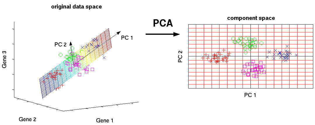
The principal component method (PCA) converts the basic features into new ones, each of which is a linear combination of the original ones in such a way that the spread of data (that is, the standard deviation from the mean value) along them is maximum. The method is used to visualize data and to reduce data dimension (compression).
For greater clarity, we randomly select 1000 objects from a training sample and draw them in the space of the first two features.
Obviously, the objects are mixed and to select among them groups of objects belonging to the same class is problematic. We will transform the data using the principal component method and draw the first two components in space. I note that the components are arranged in descending order, depending on the spread of data that falls along them.
Obviously, even in the space of only two signs, it is already possible to select explicit groups of objects. Now consider the same data, but in the space of the first three components.
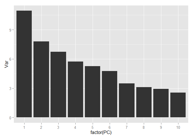
Allocation of various classes is even easier. Now select the number of components that we will use for further work. To do this, look at the ratio of the variance and the number of components explaining it, but using the entire training sample.
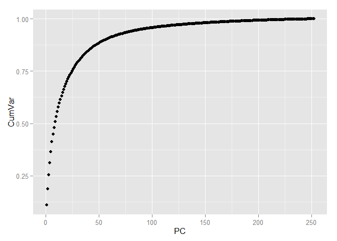
In order to save more than 90 percent of the information contained in the data, only 70 components are sufficient, i.e. we have come from 784 signs to 70 and, at the same time, have lost less than 10 percent of the data variation!
We transform the training and test samples into the space of the main components.
To select model parameters, I use the caret package, which provides the ability to perform parallel computations using the multi-core processors of today.
Now let's start creating predictive models using transformed data. Create the first model using the k-nearest-neighbor ( KNN ) method. In this model, there is only one parameter - the number of nearby objects used to classify an object. We will select this parameter using tenfold cross-validation ( 10-fold cross-validation (CV) ) with the sample split into 10 parts. Evaluation is made on a randomly selected part of the original objects. To assess the quality of the models, we will use the Accuracy metric, which is the percentage of exactly predicted classes of objects.
Now reduce it and get the exact value.
The model has the best indicator when the value of the parameter k is equal to 3. Using this value, we obtain the prediction on the test data. Construct the Confusion Table and calculate Accuracy .
The second model is Random Forest . In this model, we will choose the parameter mtry - the number of signs used when obtaining each of the trees used in the ensemble. To select the best value of this parameter, let's go the same way as before.
Select mtry equal to 4 and get Accuracy on the test data. I note that I had to train the model apart from the available training data, since to use all the data requires more RAM. But, as shown in the previous work, it does not greatly affect the final result.
And finally, Support Vector Machine . In this model, Radial Kernel will be used and two parameters are already selected: sigma (regularization parameter) and C (parameter defining the shape of the core).
Create a fourth model, which is an ensemble of three models created earlier. This model predicts the value for which most of the models used “vote”.
The following results were obtained on the test sample:
The best Accuracy indicator has a model using the k-nearest-neighbor method ( KNN ).
Evaluation of the models on the Kaggle website is given in the following table.
And the best results here are at SVM.
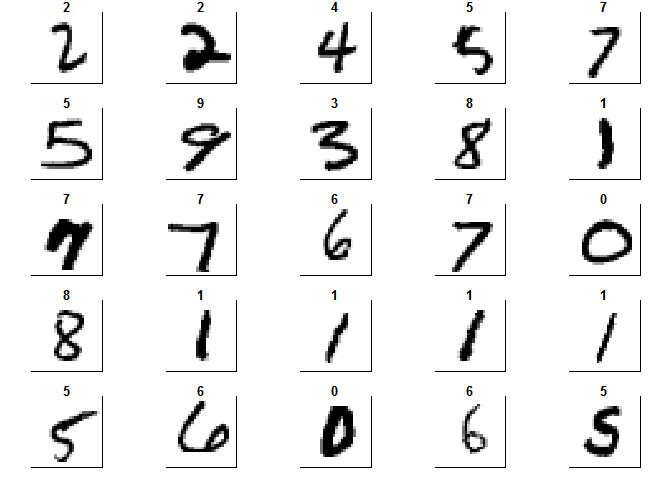
And finally, out of pure curiosity, we will visually look at the transformations produced by the method of principal components. To do this, first we get the image of the numbers in their original form.
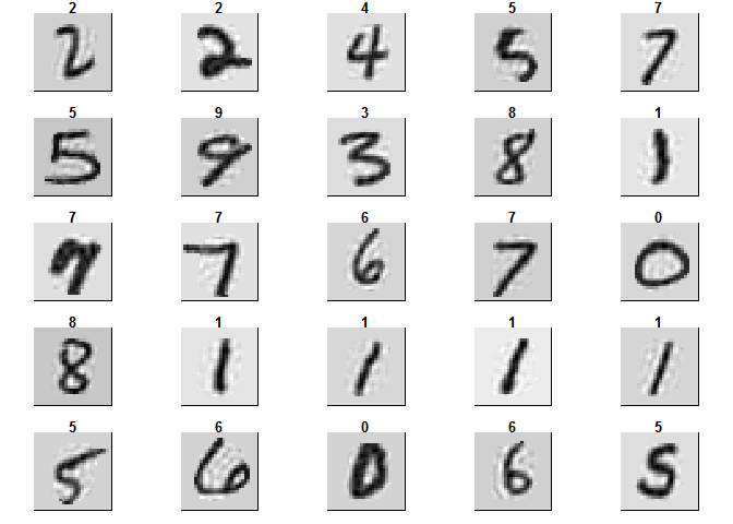
And the image of the same figures, but after we used the PCA method and left the first 70 components. The resulting objects are called eigenfaces
Next time we will consider one of the tasks of Text Mining, but for now, you can join the course on Practical Data Analysis - I recommend!
As promised, I continue to publish the analysis of tasks that I resolved while working with the guys from MLClass.ru . This time, we will analyze the principal component method using the example of the well-known digit recognition task Digit Recognizer from the Kaggle platform. The article will be useful for beginners who are just beginning to study data analysis. By the way, it is not too late to enroll in the course Applied data analysis , having the opportunity to pump as quickly as possible in this area.
Introduction
This paper is a natural continuation of the study that studies the dependence of the quality of the model on the sample size. It showed the possibility of reducing the number of objects used in the training sample in order to obtain acceptable results in conditions of limited computing resources. But, besides the number of objects, the number of features used also affects the size of the data. Consider this feature on the same data. The data used was studied in detail in previous work, so we simply load the training sample into R.
')
library(readr) library(caret) library(ggbiplot) library(ggplot2) library(dplyr) library(rgl) data_train <- read_csv("train.csv") ## |================================================================================| 100% 73 MB As we already know, the data has 42000 objects and 784 signs, representing the brightness value of each of the pixels of the figure constituting the image. Divide the sample into a training and test in the ratio of 60/40.
set.seed(111) split <- createDataPartition(data_train$label, p = 0.6, list = FALSE) train <- slice(data_train, split) test <- slice(data_train, -split) Now we remove the attributes that have a constant value.
zero_var_col <- nearZeroVar(train, saveMetrics = T) train <- train[, !zero_var_col$nzv] test <- test[, !zero_var_col$nzv] dim(train) ## [1] 25201 253 As a result, 253 signs remained.
Theory
The principal component method (PCA) converts the basic features into new ones, each of which is a linear combination of the original ones in such a way that the spread of data (that is, the standard deviation from the mean value) along them is maximum. The method is used to visualize data and to reduce data dimension (compression).
PCA
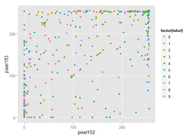
For greater clarity, we randomly select 1000 objects from a training sample and draw them in the space of the first two features.
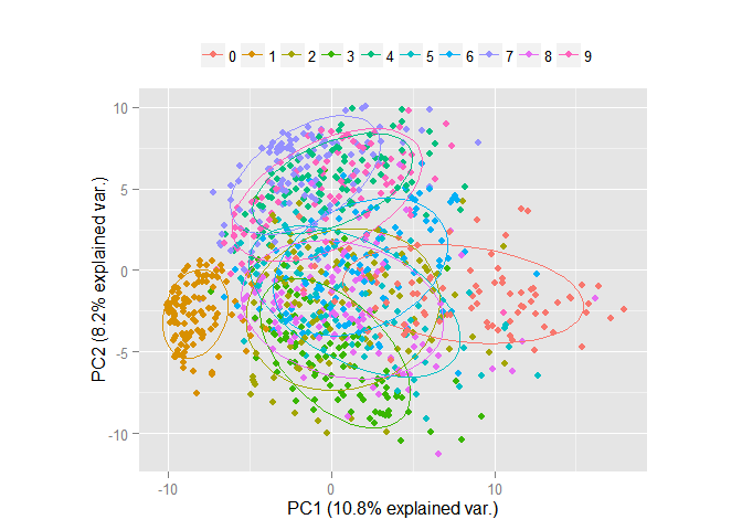
train_1000 <- train[sample(nrow(train), size = 1000),] ggplot(data = train_1000, aes(x = pixel152, y = pixel153, color = factor(label))) + geom_point() Obviously, the objects are mixed and to select among them groups of objects belonging to the same class is problematic. We will transform the data using the principal component method and draw the first two components in space. I note that the components are arranged in descending order, depending on the spread of data that falls along them.
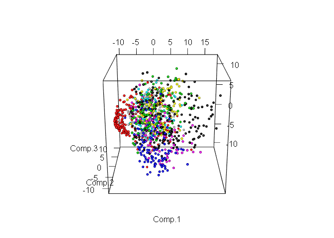
pc <- princomp(train_1000[, -1], cor=TRUE, scores=TRUE) ggbiplot(pc, obs.scale = 1, var.scale = 1, groups = factor(train_1000$label), ellipse = TRUE, circle = F, var.axes = F) + scale_color_discrete(name = '') + theme(legend.direction = 'horizontal', legend.position = 'top') Obviously, even in the space of only two signs, it is already possible to select explicit groups of objects. Now consider the same data, but in the space of the first three components.
plot3d(pc$scores[,1:3], col= train_1000$label + 1, size = 0.7, type = "s") Allocation of various classes is even easier. Now select the number of components that we will use for further work. To do this, look at the ratio of the variance and the number of components explaining it, but using the entire training sample.
pc <- princomp(train[, -1], cor=TRUE, scores=TRUE) variance <- pc$sdev^2/sum(pc$sdev^2) cumvar <- cumsum(variance) cumvar <- data.frame(PC = 1:252, CumVar = cumvar) ggplot(data = cumvar, aes(x = PC, y = CumVar)) + geom_point() variance <- data.frame(PC = 1:252, Var = variance*100) ggplot(data = variance[1:10,], aes(x = factor(PC), y = Var)) + geom_bar(stat = "identity") sum(variance$Var[1:70]) ## [1] 92.69142 In order to save more than 90 percent of the information contained in the data, only 70 components are sufficient, i.e. we have come from 784 signs to 70 and, at the same time, have lost less than 10 percent of the data variation!
We transform the training and test samples into the space of the main components.
train <- predict(pc) %>% cbind(train$label, .) %>% as.data.frame(.) %>% select(1:71) colnames(train)[1]<- "label" train$label <- as.factor(train$label) test %<>% predict(pc, .) %>% cbind(test$label, .) %>% as.data.frame(.) %>% select(1:71) colnames(test)[1]<- "label" To select model parameters, I use the caret package, which provides the ability to perform parallel computations using the multi-core processors of today.
library("doParallel") cl <- makePSOCKcluster(2) registerDoParallel(cl) Knn
Now let's start creating predictive models using transformed data. Create the first model using the k-nearest-neighbor ( KNN ) method. In this model, there is only one parameter - the number of nearby objects used to classify an object. We will select this parameter using tenfold cross-validation ( 10-fold cross-validation (CV) ) with the sample split into 10 parts. Evaluation is made on a randomly selected part of the original objects. To assess the quality of the models, we will use the Accuracy metric, which is the percentage of exactly predicted classes of objects.
set.seed(111) train_1000 <- train[sample(nrow(train), size = 1000),] ctrl <- trainControl(method="repeatedcv",repeats = 3) . knnFit <- train(label ~ ., data = train_1000, method = "knn", trControl = ctrl,tuneLength = 20) knnFit ## k-Nearest Neighbors ## ## 1000 samples ## 70 predictor ## 10 classes: '0', '1', '2', '3', '4', '5', '6', '7', '8', '9' ## ## No pre-processing ## Resampling: Cross-Validated (10 fold, repeated 3 times) ## Summary of sample sizes: 899, 901, 900, 901, 899, 899, ... ## Resampling results across tuning parameters: ## ## k Accuracy Kappa Accuracy SD Kappa SD ## 5 0.8749889 0.8608767 0.03637257 0.04047629 ## 7 0.8679743 0.8530101 0.03458659 0.03853048 ## 9 0.8652707 0.8500155 0.03336461 0.03713965 ## 11 0.8529954 0.8363199 0.03692823 0.04114777 ## 13 0.8433141 0.8255274 0.03184725 0.03548771 ## 15 0.8426833 0.8248052 0.04097424 0.04568565 ## 17 0.8423694 0.8244683 0.04070299 0.04540152 ## 19 0.8340150 0.8151256 0.04291349 0.04788273 ## 21 0.8263450 0.8065723 0.03914363 0.04369889 ## 23 0.8200042 0.7995067 0.03872017 0.04320466 ## 25 0.8156764 0.7946582 0.03825163 0.04269085 ## 27 0.8093227 0.7875839 0.04299301 0.04799252 ## 29 0.8010018 0.7783100 0.04252630 0.04747852 ## 31 0.8019849 0.7794036 0.04327120 0.04827493 ## 33 0.7963572 0.7731147 0.04418378 0.04930341 ## 35 0.7936906 0.7701616 0.04012802 0.04478789 ## 37 0.7889930 0.7649252 0.04163075 0.04644193 ## 39 0.7863463 0.7619669 0.03947693 0.04404655 ## 41 0.7829758 0.7582087 0.03482612 0.03889550 ## 43 0.7796388 0.7544879 0.03745359 0.04179976 ## ## Accuracy was used to select the optimal model using the largest value. ## The final value used for the model was k = 5. Now reduce it and get the exact value.
grid <- expand.grid(k=2:5) knnFit <- train(label ~ ., data = train_1000, method = "knn", trControl = ctrl, tuneGrid=grid) knnFit ## k-Nearest Neighbors ## ## 1000 samples ## 70 predictor ## 10 classes: '0', '1', '2', '3', '4', '5', '6', '7', '8', '9' ## ## No pre-processing ## Resampling: Cross-Validated (10 fold, repeated 3 times) ## Summary of sample sizes: 900, 901, 901, 899, 901, 899, ... ## Resampling results across tuning parameters: ## ## k Accuracy Kappa Accuracy SD Kappa SD ## 2 0.8699952 0.8553199 0.03055544 0.03402108 ## 3 0.8799832 0.8664399 0.02768544 0.03082014 ## 4 0.8736591 0.8593777 0.02591618 0.02888557 ## 5 0.8726753 0.8582703 0.02414173 0.02689738 ## ## Accuracy was used to select the optimal model using the largest value. ## The final value used for the model was k = 3. The model has the best indicator when the value of the parameter k is equal to 3. Using this value, we obtain the prediction on the test data. Construct the Confusion Table and calculate Accuracy .
library(class) prediction_knn <- knn(train, test, train$label, k=3) table(test$label, prediction_knn) ## prediction_knn ## 0 1 2 3 4 5 6 7 8 9 ## 0 1643 0 6 1 0 1 2 0 0 0 ## 1 0 1861 4 1 2 0 0 0 0 0 ## 2 7 7 1647 3 0 0 1 11 0 0 ## 3 1 0 9 1708 2 19 4 6 1 3 ## 4 0 4 0 0 1589 0 10 7 0 6 ## 5 3 2 1 20 1 1474 13 0 6 2 ## 6 0 0 0 1 2 3 1660 0 0 0 ## 7 0 6 3 0 2 0 0 1721 0 13 ## 8 0 1 0 11 1 16 12 4 1522 20 ## 9 0 0 1 3 3 5 1 23 5 1672 sum(diag(table(test$label, prediction_knn)))/nrow(test) ## [1] 0.9820227 Random forest
The second model is Random Forest . In this model, we will choose the parameter mtry - the number of signs used when obtaining each of the trees used in the ensemble. To select the best value of this parameter, let's go the same way as before.
rfFit <- train(label ~ ., data = train_1000, method = "rf", trControl = ctrl,tuneLength = 3) rfFit ## Random Forest ## ## 1000 samples ## 70 predictor ## 10 classes: '0', '1', '2', '3', '4', '5', '6', '7', '8', '9' ## ## No pre-processing ## Resampling: Cross-Validated (10 fold, repeated 3 times) ## Summary of sample sizes: 901, 900, 900, 899, 902, 899, ... ## Resampling results across tuning parameters: ## ## mtry Accuracy Kappa Accuracy SD Kappa SD ## 2 0.8526986 0.8358081 0.02889351 0.03226317 ## 36 0.8324051 0.8133909 0.03442843 0.03836844 ## 70 0.8026823 0.7802912 0.03696172 0.04118363 ## ## Accuracy was used to select the optimal model using the largest value. ## The final value used for the model was mtry = 2. grid <- expand.grid(mtry=2:6) rfFit <- train(label ~ ., data = train_1000, method = "rf", trControl = ctrl,tuneGrid=grid) rfFit ## Random Forest ## ## 1000 samples ## 70 predictor ## 10 classes: '0', '1', '2', '3', '4', '5', '6', '7', '8', '9' ## ## No pre-processing ## Resampling: Cross-Validated (10 fold, repeated 3 times) ## Summary of sample sizes: 898, 900, 900, 901, 900, 898, ... ## Resampling results across tuning parameters: ## ## mtry Accuracy Kappa Accuracy SD Kappa SD ## 2 0.8553016 0.8387134 0.03556811 0.03967709 ## 3 0.8615798 0.8457973 0.03102887 0.03458732 ## 4 0.8669329 0.8517297 0.03306870 0.03690844 ## 5 0.8739532 0.8595897 0.02957395 0.03296439 ## 6 0.8696883 0.8548470 0.03203166 0.03568138 ## ## Accuracy was used to select the optimal model using the largest value. ## The final value used for the model was mtry = 5. Select mtry equal to 4 and get Accuracy on the test data. I note that I had to train the model apart from the available training data, since to use all the data requires more RAM. But, as shown in the previous work, it does not greatly affect the final result.
library(randomForest) rfFit <- randomForest(label ~ ., data = train[sample(nrow(train), size = 15000),], mtry = 4) prediction_rf<-predict(rfFit,test) table(test$label, prediction_rf) ## prediction_rf ## 0 1 2 3 4 5 6 7 8 9 ## 0 1608 0 6 3 4 1 20 2 9 0 ## 1 0 1828 9 9 3 5 3 2 9 0 ## 2 12 9 1562 16 15 5 6 19 31 1 ## 3 12 1 26 1625 2 33 12 14 22 6 ## 4 0 6 11 1 1524 0 22 7 6 39 ## 5 12 3 3 48 12 1415 10 1 15 3 ## 6 13 4 8 0 4 11 1623 0 3 0 ## 7 3 14 25 2 13 3 0 1653 4 28 ## 8 4 10 12 64 8 21 12 5 1428 23 ## 9 4 4 10 39 38 10 0 39 7 1562 sum(diag(table(test$label, prediction_rf)))/nrow(test) ## [1] 0.9421989 SVM
And finally, Support Vector Machine . In this model, Radial Kernel will be used and two parameters are already selected: sigma (regularization parameter) and C (parameter defining the shape of the core).
svmFit <- train(label ~ ., data = train_1000, method = "svmRadial", trControl = ctrl,tuneLength = 5) svmFit ## Support Vector Machines with Radial Basis Function Kernel ## ## 1000 samples ## 70 predictor ## 10 classes: '0', '1', '2', '3', '4', '5', '6', '7', '8', '9' ## ## No pre-processing ## Resampling: Cross-Validated (10 fold, repeated 3 times) ## Summary of sample sizes: 901, 900, 898, 900, 900, 901, ... ## Resampling results across tuning parameters: ## ## C Accuracy Kappa Accuracy SD Kappa SD ## 0.25 0.7862419 0.7612933 0.02209354 0.02469667 ## 0.50 0.8545924 0.8381166 0.02931921 0.03262332 ## 1.00 0.8826064 0.8694079 0.02903226 0.03225475 ## 2.00 0.8929180 0.8808766 0.02781461 0.03090255 ## 4.00 0.8986322 0.8872208 0.02607149 0.02898200 ## ## Tuning parameter 'sigma' was held constant at a value of 0.007650572 ## Accuracy was used to select the optimal model using the largest value. ## The final values used for the model were sigma = 0.007650572 and C = 4. grid <- expand.grid(C = 4:6, sigma = seq(0.006, 0.009, 0.001)) svmFit <- train(label ~ ., data = train_1000, method = "svmRadial", trControl = ctrl,tuneGrid=grid) svmFit ## Support Vector Machines with Radial Basis Function Kernel ## ## 1000 samples ## 70 predictor ## 10 classes: '0', '1', '2', '3', '4', '5', '6', '7', '8', '9' ## ## No pre-processing ## Resampling: Cross-Validated (10 fold, repeated 3 times) ## Summary of sample sizes: 901, 900, 900, 899, 901, 901, ... ## Resampling results across tuning parameters: ## ## C sigma Accuracy Kappa Accuracy SD Kappa SD ## 4 0.006 0.8943835 0.8824894 0.02999785 0.03335171 ## 4 0.007 0.8970537 0.8854531 0.02873482 0.03194698 ## 4 0.008 0.8984139 0.8869749 0.03068411 0.03410783 ## 4 0.009 0.8990838 0.8877269 0.03122154 0.03469947 ## 5 0.006 0.8960834 0.8843721 0.03061547 0.03404636 ## 5 0.007 0.8960703 0.8843617 0.03069610 0.03412880 ## 5 0.008 0.8990774 0.8877134 0.03083329 0.03427321 ## 5 0.009 0.8990838 0.8877271 0.03122154 0.03469983 ## 6 0.006 0.8957534 0.8840045 0.03094360 0.03441242 ## 6 0.007 0.8963971 0.8847267 0.03081294 0.03425451 ## 6 0.008 0.8990774 0.8877134 0.03083329 0.03427321 ## 6 0.009 0.8990838 0.8877271 0.03122154 0.03469983 ## ## Accuracy was used to select the optimal model using the largest value. ## The final values used for the model were sigma = 0.009 and C = 4. library(kernlab) svmFit <- ksvm(label ~ ., data = train,type="C-svc",kernel="rbfdot",kpar=list(sigma=0.008),C=4) prediction_svm <- predict(svmFit, newdata = test) table(test$label, prediction_svm) ## prediction_svm ## 0 1 2 3 4 5 6 7 8 9 ## 0 1625 0 5 1 0 3 13 0 6 0 ## 1 1 1841 6 6 4 1 0 3 5 1 ## 2 8 4 1624 5 7 1 1 13 11 2 ## 3 2 0 18 1684 0 23 2 6 12 6 ## 4 1 3 3 0 1567 0 9 7 5 21 ## 5 8 3 2 24 6 1465 7 0 6 1 ## 6 2 1 2 1 5 5 1649 0 1 0 ## 7 3 8 15 3 3 0 0 1695 3 15 ## 8 1 6 10 10 5 9 3 4 1530 9 ## 9 3 1 5 13 14 9 0 21 3 1644 sum(diag(table(test$label, prediction_svm)))/nrow(test) ## [1] 0.9717245 Model Ensemble
Create a fourth model, which is an ensemble of three models created earlier. This model predicts the value for which most of the models used “vote”.
all_prediction <- cbind(as.numeric(levels(prediction_knn))[prediction_knn], as.numeric(levels(prediction_rf))[prediction_rf], as.numeric(levels(prediction_svm))[prediction_svm]) predictions_ensemble <- apply(all_prediction, 1, function(row) { row %>% table(.) %>% which.max(.) %>% names(.) %>% as.numeric(.) }) table(test$label, predictions_ensemble) ## predictions_ensemble ## 0 1 2 3 4 5 6 7 8 9 ## 0 1636 0 5 1 0 1 8 0 2 0 ## 1 1 1851 3 5 3 0 0 1 4 0 ## 2 7 6 1636 3 6 0 0 11 7 0 ## 3 6 0 14 1690 1 18 4 8 7 5 ## 4 0 5 4 0 1573 0 12 6 2 14 ## 5 5 1 2 21 5 1478 7 0 3 0 ## 6 3 1 2 0 5 3 1651 0 1 0 ## 7 1 11 12 2 1 0 0 1704 0 14 ## 8 1 5 11 17 4 13 4 3 1514 15 ## 9 4 2 4 21 11 5 0 20 1 1645 sum(diag(table(test$label, predictions_ensemble)))/nrow(test) ## [1] 0.974939 Results
The following results were obtained on the test sample:
| Model | Test accuracy |
| Knn | 0.981 |
| Random forest | 0.948 |
| SVM | 0.971 |
| Ensemble | 0.974 |
The best Accuracy indicator has a model using the k-nearest-neighbor method ( KNN ).
Evaluation of the models on the Kaggle website is given in the following table.
| Model | Kaggle Accuracy |
| Knn | 0.97171 |
| Random forest | 0.93286 |
| SVM | 0.97786 |
| Ensemble | 0.97471 |
And the best results here are at SVM.
Eigenfaces
And finally, out of pure curiosity, we will visually look at the transformations produced by the method of principal components. To do this, first we get the image of the numbers in their original form.
set.seed(100) train_1000 <- data_train[sample(nrow(data_train), size = 1000),] colors<-c('white','black') cus_col<-colorRampPalette(colors=colors) default_par <- par() number_row <- 28 number_col <- 28 par(mfrow=c(5,5),pty='s',mar=c(1,1,1,1),xaxt='n',yaxt='n') for(i in 1:25) { z<-array(as.matrix(train_1000)[i,-1],dim=c(number_row,number_col)) z<-z[,number_col:1] image(1:number_row,1:number_col,z,main=train_1000[i,1],col=cus_col(256)) } par(default_par) And the image of the same figures, but after we used the PCA method and left the first 70 components. The resulting objects are called eigenfaces
zero_var_col <- nearZeroVar(train_1000, saveMetrics = T) train_1000_cut <- train_1000[, !zero_var_col$nzv] pca <- prcomp(train_1000_cut[, -1], center = TRUE, scale = TRUE) restr <- pca$x[,1:70] %*% t(pca$rotation[,1:70]) restr <- scale(restr, center = FALSE , scale=1/pca$scale) restr <- scale(restr, center = -1 * pca$center, scale=FALSE) restr <- as.data.frame(cbind(train_1000_cut$label, restr)) test <- data.frame(matrix(NA, nrow = 1000, ncol = ncol(train_1000))) zero_col_number <- 1 for (i in 1:ncol(train_1000)) { if (zero_var_col$nzv[i] == F) { test[, i] <- restr[, zero_col_number] zero_col_number <- zero_col_number + 1 } else test[, i] <- train_1000[, i] } par(mfrow=c(5,5),pty='s',mar=c(1,1,1,1),xaxt='n',yaxt='n') for(i in 1:25) { z<-array(as.matrix(test)[i,-1],dim=c(number_row,number_col)) z<-z[,number_col:1] image(1:number_row,1:number_col,z,main=test[i,1],col=cus_col(256)) } par(default_par) Next time we will consider one of the tasks of Text Mining, but for now, you can join the course on Practical Data Analysis - I recommend!
Source: https://habr.com/ru/post/267075/
All Articles