The time series forecasting model for the maximum similarity sample: an explanation and an example

Foreword

This is my model. I invented it, programmatically implemented it, studied the features and described it. The resulting description was defended as a thesis on the topic “Time Series Forecasting Model for a Sample of Maximum Similarity” . The developed model belongs to the class of statistical forecasting models and builds a forecast of the time series based on the actual values ​​of the same series. More information about the classification I wrote earlier. One of the modifications of the model allows you to take into account the influence of external factors on the forecast.

Files with the implemented example can be downloaded in the archive .

UPD 03/07/2019 : An updated version of the sample for MATLAB 2015b is available with comments in English .

1. Explanation of the prediction model for the maximum similarity sample

1.1. The main idea and its illustration on time series samples

A complete formal description of the prediction model can be found in the second chapter of my thesis. However, speaking simply, the model is based on the idea of ​​the development of history in a spiral: the stages are repeated, but with varying properties.

If we apply this idea to the time series, then we can say this: in the actual values ​​of the time series, if there are enough of them, there is surely a segment that is very similar to what happens on the eve of the forecast.

In fig. Figure 1 shows a part of the time series Z (t), for which similar segments are noticeable without special calculations. Let us call the time series segment beginning at time mark t and the length (number of samples) M, the time series pattern of the time series and denote Z ^M _t .

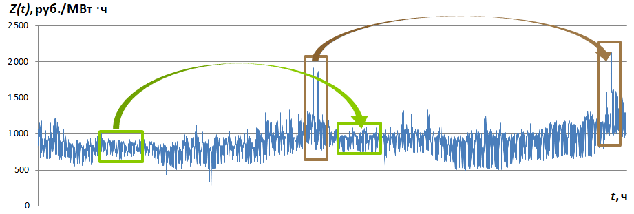
Fig. 1. The time series Z (t) and some of its samples

Every forecasting model comes from some assumption. In the model of the maximum similarity sample, it is assumed that if history repeats, then for each sample preceding the forecast there is a similar sample contained in the actual values ​​of the same time series. Formally, this is called the similarity hypothesis (see dissertation).

The ratio of samples and their name can be seen in Fig. 2

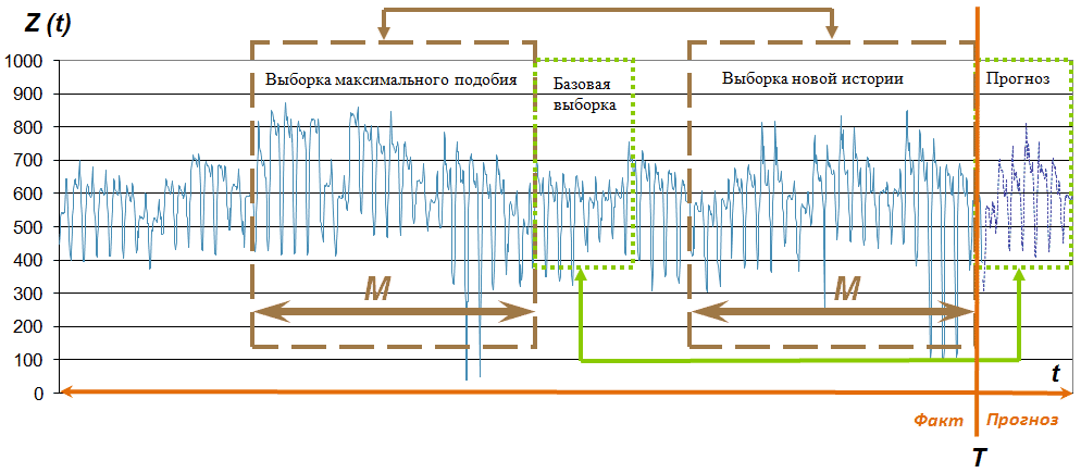
Fig. 2. Sampling time series Z (t)

At time T, which is called the forecast time , you need to determine the P values ​​of the time series in the future, i.e., calculate the Projection sample. At the same time, the values ​​of the New history selection are available. Further, based on the assumption that there is a similar one for each sample, you need to find the Maximum similarity sample for the New history sample and assume that the history will repeat, that is, the Basic sample will be the basis for the predicted values.

Next, you need to answer three questions.

1.2. How to determine the similarity of samples?

In my dissertation, I propose the simplest version of the definition of similarity — the calculation of the linear correlation value . Take one sample of length M, take another sample of length M, read the correlation value, which will reflect the similarity of the two samples.

Search for the sample of maximum similarity is the easiest way to search among all possible samples. For time series up to 100,000 values ​​of this sort, brute force takes a few seconds when implemented on a personal computer of average power.

The proposed approach of determining similarity is not the only possible one. A number of students-followers offered in their work other methods for determining the similarity of two samples. You can apply your imagination here!

1.3. How to "transfer" the change of properties?

Due to the fact that the basis of the similarity definition is based on a linear correlation, the simplest way to “transfer” the properties of the samples is the linear dependence

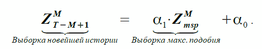(one)

If equation (1) reflects the dependence of two actual samples using coefficients α ₁ and α ₀ , then on the basis of the assumption of similarity, the Forecast and Basic sample are correlated as follows:

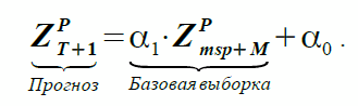(2)

The coefficients α ₁ and α ₀ in both equations are the same, but for equation (1) they are unknown and need to be determined, and for equation (2) they are known. The msp index stands for the most similar pattern .

The model name in English sounds like extrapolation (or forecast) model on the most most similar pattern, abbreviated EMMSP.

1.4. Does the assumption of similarity always work?

This needs to be checked for each new task. Every time series model is a tool for handling this series, and, like any tool, the model must be used properly. Roughly speaking, you need to hammer in nails and dig the ground with a shovel, and not vice versa.

The developed model showed excellent results in the tasks of short-term forecasting of time series in the field of electric power industry , where it is necessary to predict prices and volumes of energy consumption. The model showed results comparable to the results of other forecasting models on financial time series, blood sugar level, etc. Numerical values ​​of errors can be found in the fourth chapter of the thesis and a set of reports on the prediction of indicators of the wholesale electricity and capacity market .

The most important property of the proposed model is its simplicity and clarity.

2. An example of the implementation of the prediction model for the sample of maximum similarity in MATLAB

An example of a prediction model is implemented in MATLAB.

2.1. Initial data, formulation of the prediction problem and model parameters

The initial data are the values ​​of electricity prices in the European territory of the Russian Federation of the wholesale electricity and capacity market in rubles / MW • h from 01/09/2006 to 13/11/2012 at hourly rates. The PRICES_EUR archive contains 54,384 values.

It is necessary to calculate the forecast of this time series at P = 24 values ​​ahead, i.e., one day ahead at the time of the forecast T = 09/01/2012 23:00:00.

Loading raw data:

%           %   ,  PRICES_EUR    % <Date> - <Hour> - <Value> load PRICES_EUR PRICES_EUR; %      PRICES_EUR.mat TimeSeries = PRICES_EUR; 

Statement of the forecasting task:

 %    T = datenum('01.09.2012 23:00:00', 'dd.mm.yyyy hh:MM:ss'); %   (Origin) P = 24; %   (Forecast horizon) 

Parameters of the EMMSP prediction model:

 %       M = 144; Step = 24; 

In this case, the length of the sample of the new history and the sample of maximum similarity is M = 144. Read more about how to define M, read the third chapter of the thesis .

The step variable is a step of iterating over the actual values ​​when determining the maximum similarity sample .

2.2. Algorithm prediction model for a sample of maximum similarity

2.2.1. Define a sample of new history

')

 Index = find(TimeSeries(:,1) == datenum(year(T), month(T), day(T)) & TimeSeries(:,2) == hour(T)); if length(Index) > 1 fprintf(['  :   T      1  \n']); elseif isempty(Index) fprintf(['  :   T      \n']); else HistNewData = TimeSeries([Index-M+1:Index],:); %    (HistNewData) Index = Index - Step * 2; end 

2.2.2. Determine the similarity values

 k = 1; while Index > 2 * M HistOldData = TimeSeries([Index-M+1 : Index],:); Likeness(k,1)= Index; CheckOld = find(HistOldData(:,3) > 0); %   ,    CheckNew = find(HistNewData(:,3) > 0); if isempty(CheckOld) || isempty(CheckNew) Likeness(k,2) = 0; else Likeness(k,2) = abs(corr(HistOldData(:,3), HistNewData(:,3), 'type', 'Pearson')); end k = k + 1; Index = Index - Step; %       Step end 

The step of iteration Step = 24 is taken from the consideration that the time series has a pronounced daily frequency.

2.2.3. Define maximum similarity

 MaxLikeness = max(abs(Likeness(:,2))); IndexLikeness = find(Likeness(:,2) == MaxLikeness); MSP = Likeness(IndexLikeness(1),1); 

Practice shows that there can be several maximums of similarity. The most convenient is to take the first.

2.2.4. Determine the maximum similarity sample

 MSPData = TimeSeries([MSP-M+1 : MSP],:); %    (MSPData) 

2.2.5. Define basic sample

 HistBaseData = TimeSeries([MSP+1:MSP+P],:); %   (HistBaseData) 

2.2.6 Search for coefficients α ₁ and α ₀

 %   HistNewData   MSPData    . %        . %      ,      . X = MSPData(:,3); X(:,length(X(1,:))+1) = 1; %      I Y = HistNewData(:,3); E = X(:,2); Xn = X'* X; Yn = X'* Y; invX = inv(Xn); A = invX * Yn; %   alpha1  alpha0    A 

After finding the values ​​of the coefficients α ₁ and α _0, you can check with which error the Sample of the new history is similar to the Sample of maximum similarity , that is, what is the error of equation (1). In the present example, verification is omitted for simplicity.

2.2.7. Forecasting

 X = HistBaseData(:,3); X(:,length(X(1,:))+1) = 1; Forecast = X * A; %  ,  24   

In the implemented example, the number of predictive samples can be changed by changing the parameter P.

2.2.8. Estimation of forecasting error

 % 1)    Index = find(TimeSeries(:,1) == datenum(year(T), month(T), day(T)) & TimeSeries(:,2) == hour(T)); Fact = TimeSeries([Index : Index+P-1],3); % 2)   MAE MAE = mean(abs(Forecast - Fact)); % 3)   MAPE MAPE = mean(abs(Forecast - Fact)./Fact); fprintf(['  T = ',datestr(T,'dd.mm.yyyy HH:MM'),'\n', '  P = ', num2str(P),'\n', '  MAE = ',num2str(MAE),' RUB/MWh, MAPE = ',num2str(MAPE*100),'%% \n']); 

As a result of program execution, the following message should appear in the MATLAB command line:

   MaxLikeness = 0.95817  alpha1 = 1.0312,  alpha0 = -11.1992   T = 01.09.2012 23:00   P = 24   MAE = 57.6383 RUB/MWh, MAPE = 6.0065% 

Questions? You can ask them here if you have an account on Habré, or on our forum , if you don’t have one.