Search for periodic security elements of the RF Passport using the Fourier transform: part two
Many documents contain security features such as holograms, watermarks, guilloches, etc. In the process of scanning such documents there is a problem - the security elements interfere with the recognition systems (OCR). In developing Smart PassportReader, we conducted a study aimed at finding and eliminating similar security elements from document images.

In our previous article on this topic, we talked about the first half of the search problem solution — detection, i.e. determining the presence of periodic elements in the image. Today we will tell how to find the immediate position of the periodic elements in the image, provided that the detection was successful: we are sure that the elements in the image are present. The second part depends heavily on the first, so it is strongly recommended that you first get acquainted with the first, if you have not already done so.
')
Like last time, the Fourier transform will be used for this.
Like last time, many arguments will be shown for the one-dimensional case, which is then easily transferred to the two-dimensional one.
Recall that) - original image length
- original image length  consisting of two others: background image
 ) and images
and images ) containing a periodic pattern. Picture in turn, we presented a single instance of the template convolution
containing a periodic pattern. Picture in turn, we presented a single instance of the template convolution ) with Dirac's crest
with Dirac's crest ) :
:
%20%3D%20h(x)%20%2B%20g(x)%20%3D%20h(x)%20%2B%20f(x)%20%5Cast%20c(x))
Since we know in advance the structure of the periodic pattern (in the case of the RF passport, the size and period of the holograms), to restore the position of the elements, it is enough to know only the horizontal and vertical shift of the entire template, which is the same as the shift of one of the “eagles”.
Shift signal pattern equivalent to impulse shift which leads to a modified form ) . The spectrum of the Fourier transform of the shifted signal changes only in phase, leaving the amplitude unchanged, thereby allowing the periodic patterns to be detected independently of their initial shift. As an important consequence, all the useful phase information is concentrated in the same DFT positions (frequencies) as the amplitudes of the pulsed signal.
. The spectrum of the Fourier transform of the shifted signal changes only in phase, leaving the amplitude unchanged, thereby allowing the periodic patterns to be detected independently of their initial shift. As an important consequence, all the useful phase information is concentrated in the same DFT positions (frequencies) as the amplitudes of the pulsed signal.
Let's pretend that shifted to the right by  , then:
%20%3D%20%5Cmathcal%7BF%7D_k%20c(x)%20%5Ccdot%20e%5E%7Bi%20%5CPhi_k%7D%2C)

Since the phase angle) for unbiased equals zero for offset
for unbiased equals zero for offset ) he becomes equal
he becomes equal  . To obtain a phase shift
 ) we need to add each member to the corresponding phase angle in
we need to add each member to the corresponding phase angle in ) for each
for each  . Note that any phase angle is always taken modulo
  and is limited by the interval
 ) .
.
Phase shift on in the frequency domain represents the shift in the time domain but has a period  , so we can avoid redundancy by considering only
  thus ensuring
  . For convenience, let
  Is a phase shift in which corresponds to the time shift by
  and also let
  Is the phase angle on
  Amplitude peak:

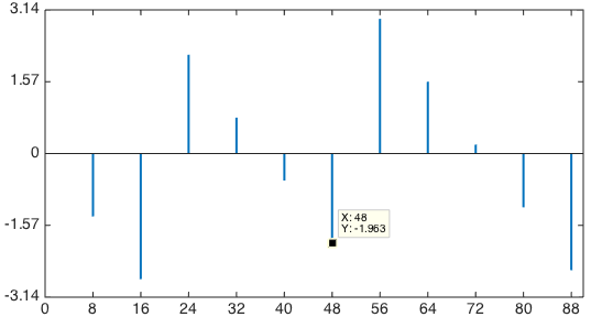
The figure shows an example of the DFT phase of a shifted pulsed signal with values period
  and shift
  . For example,
  and
and %20%5Ccdot%206%20%5Capprox%20-1%2C963) .
.
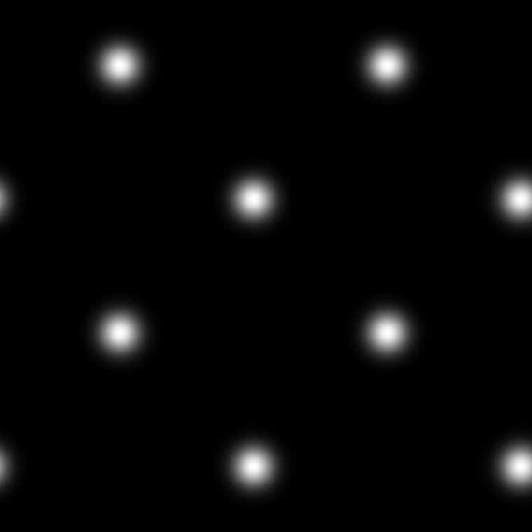
And this is how the amplitude and phase of the DFT looks like for a Gaussian grid like a chessboard:
 - DFT ->

For a two-dimensional image, the phase shift now consists of two components ) . We introduce a coordinate grid for the DFT of a chess-like system of peaks shown in the second and third figures above, such that the central peak has coordinates
. We introduce a coordinate grid for the DFT of a chess-like system of peaks shown in the second and third figures above, such that the central peak has coordinates ) peaks right above
peaks right above ) ,
, ) and so on; the nearest diagonal peak has coordinates
and so on; the nearest diagonal peak has coordinates ) . In general, the peak
. In general, the peak ) present if and only if
present if and only if ) - even.
- even.
Applying again the theorem on the DFT of a shifted signal, one can extend the shift equation and show that the phase angle on The peak for a two-dimensional pulse signal is:

As for the one-dimensional case, to obtain a shifted phase) need to add to the appropriate phase
need to add to the appropriate phase ) .
.
To determine the exact location of the periodic pattern, it is sufficient to estimate its phase shift.) since its pixel periodic structure is known in advance. Pixel shift
since its pixel periodic structure is known in advance. Pixel shift ) , subsequently, it is not difficult to recover from the information on the phase shift.
, subsequently, it is not difficult to recover from the information on the phase shift.
In the first article, we described the different stages of preprocessing the original image of a passport. First, an area containing a 2x2 grid (similar to a chessboard) and containing 2 patterns horizontally and vertically is cut out of the image. This can be done (with an error of less than 5%), since the physical dimensions of the document, the size and period of the periodic patterns are fixed and known in advance. The position of the region can be set by combining the physical coordinates of the document with its coordinates in the image.
Next, a significant compression and smoothing of the image is performed to suppress the background and to level the differences between the periodic patterns. The figure below shows an image of a cut-out region of a Russian passport, the results of its preprocessing and the amplitude of its DFT.
 - processing ->
 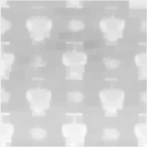 - DFT ->
As expected, the DFT amplitude has noticeable peaks with a distribution similar to a chessboard.
According to the image model, the original image consists of three independent signals: the background image and single sample periodic pattern that rolls up with a shifted pulse signal to get a periodic pattern :
%20%3D%20h(x)%20%2B%20f(x)%20*%20c(x)%0A)
After performing the DFT on , we have:
%20%3D%20%5Cmathcal%7BF%7D%20h(x)%20%2B%20%5Cmathcal%7BF%7D%20f(x)%20%5Ccdot%20%5Cmathcal%7BF%7D%20c(x)%0A)
To obtain a phase shift stored in from ) , which we calculated for this image, we need to gradually suppress the other components of the equation.
, which we calculated for this image, we need to gradually suppress the other components of the equation.
If the background after preprocessing is fairly homogeneous on the documents being processed, simple calculation of the averaged spectrum is possible ) on images of documents on which there is no desired periodic pattern, with its subsequent subtraction from .
on images of documents on which there is no desired periodic pattern, with its subsequent subtraction from .
However, the background image in our model, in fact, it is not a background in terms of the structure of a Russian passport: it contains personal data, which, by definition, differ on the set to be processed.
We have previously mentioned the fact that the DFT positions (frequencies) without peaks do not contain useful information regarding periodic patterns, since they represent the background. Assuming that is smooth, we can interpolate its contribution to each peak ) based on values adjacent to peak positions. Average value
based on values adjacent to peak positions. Average value %7D) by
by ) on the nearest neighbors peak
on the nearest neighbors peak %5C%7D) 3x3 window is an acceptable estimate
3x3 window is an acceptable estimate ) to subtract from To clear out the background:
to subtract from To clear out the background:
%20%5Cleftarrow%20%5Cmathcal%7BF%7D%20I(x%2C%20y)%20-%20%5Coverline%7B%5Cmathcal%7BF%7D%20I(x'%2C%20y')%7D%0A)
The following figure contains a compressed image and an image obtained as a result of the inverse DFT after subtracting the interpolated background spectrum and resetting the DFT at all off-peak frequencies.
 - DFT, subtraction of the background spectrum, inverse DFT ---->
As expected, only the periodic pattern remained on a plain monotone background, and instances of the periodic pattern became more similar to each other. Note that the background is not black because the DFT value on The value averaged over the image has not been reset.
After removing the background spectrum, we have left%20%5Ccdot%20%5Cmathcal%7BF%7D%20c(x)) . When multiplying two complex numbers, their phases are added. Then, to reach the phase angle
. When multiplying two complex numbers, their phases are added. Then, to reach the phase angle ) at peak corresponding to the phase angle of the spectrum of a single instance of a periodic pattern
at peak corresponding to the phase angle of the spectrum of a single instance of a periodic pattern ) must be deducted.
must be deducted.
The problem is that the spectrum of the periodic pattern is usually unknown. One of the possible solutions is the experimental calculation of the phase of the presented pattern of the pattern and its subsequent subtraction. In our experiments, we used a different path, assuming that the phase contribution constant means to resultant shift one more constant shift is added. This shift constant can be estimated experimentally as a systematic error on a test dataset.
At the end of the spectrum preprocessing, we have the phase angle of the pulsed signal which presumably contains all the necessary information about the phase shift %5ET%7D) .
.
We can build a system of equations (each equation corresponds to peak) modulo :

Or, in matrix form:

The left part of the system contains the “ideal” phase values corresponding to the peaks, and the right part contains the actual value of the DFT phase for this image at the peak positions.
This system is redefined, because she has equations (by the number of peaks considered) and only 2 variables:
  and
and  . Overdetermined systems of equations can be approximately solved by the least squares (OLS) method by finding a solution that minimizes the sum of squared residuals. However, this system is a modular system. therefore, MNCs cannot be directly applied, but we can calculate the initial solution and correct it with a sequential solution of the system.
Let's look at two equations for peaks numbered and :

This system has 4 valid solutions:) ,
, ) ,
, ) and
and ) . Because of the chessboard-like structure of peak patterns in our case, and also because represents a shift by a unit period, the first with the fourth solution are identical, as well as the second with the third. Two potential solutions remain:
. Because of the chessboard-like structure of peak patterns in our case, and also because represents a shift by a unit period, the first with the fourth solution are identical, as well as the second with the third. Two potential solutions remain: %5ET) and
and %5ET) .
.
To choose the right solution, we can add to the system the two remaining equations for the peaks and ) by making the system redefined again. Then, the value of the residual
by making the system redefined again. Then, the value of the residual  calculated for th decision
  with all
  equations:
%5E2%7D%0A%20%20%20%20%20%20%20%20%20%20%20%3D%20%5Cfrac%7B1%7D%7Bn%7D%7CA%5Cphi%5E*_k-b%7C%5E2%20)
Note that intermediate calculations involving phase angles (difference calculation) are performed in) .
.
Finally, the solution the lowest value selected as  Because the other solution will have much larger residual values. Great importance for may mean false peak detection.
The initial solution found above could be good if the remaining spectrum contained only information about and nothing more. Unfortunately, it is distorted by spectral components from the background and from samples of periodic patterns that were not completely removed during the preprocessing.
At this stage, the selected solution is still true, but can be refined using phase information at different peaks, and not just for the first two. Subtract  (using equations) from both sides of the system of equations, thus moving the solution space along and getting the following overdetermined system of equations for the corrective solution
  :
:

Assuming that, in the first approximation of the solution, we were no more mistaken than , we can not take the system modulo because after shifting the system, every equation will be inside , which means that we can approximately solve the system using the least squares method. After deciding
  found, it should be added to the previously found initial solution as a correction value.
So far, we have considered equations for the first 4 peaks. having ) an amount of 2 (and
an amount of 2 (and  because of the symmetry of the DFT), but there are other peaks with sums equal to 4, 6, and so on. The reason why they were not added earlier is that when you increase the number of suitable system solutions is also increasing, and the closer they become to each other modulo .
To use the information about the phase shift contained in the remaining peaks, we can repeat the above process of adjusting the initial solution, replacing the adjusted solution obtained for an amount equal to 4 and using all equations having an amount equal to 6 and so on, until the required accuracy is achieved. Assuming that the error decreases with increasing iteration, each equation will be within That allows you to use OLS to solve the system.
Now having a phase shift , we can easily convert it back to pixel shift . Knowing the period and size of the patterns, we can restore the position of each grid pattern. The size and position of the excised region that we used in the process are also known, so we can get the position of the patterns on the original document image.
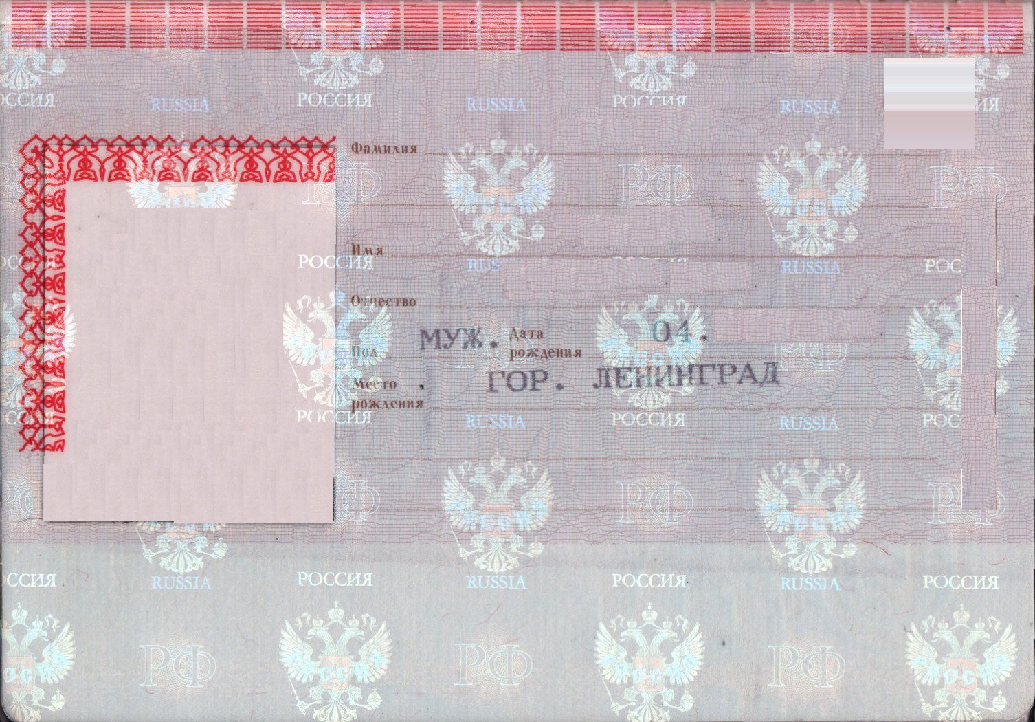
The following picture, which you have already seen at the very beginning of the article, presents an example of finding a holographic periodic pattern on a Russian passport.
A box with a circle inside indicates the result found after solving the system of equations. The other boxes indicate the extrapolated positions of the other patterns.
We used a data set of 484 images of scanned Russian passports with holographic content. For each image in the set, we prepared the true value of the pixel shift of its periodic pattern. The table below contains the experimental results for this data set with the average value of the bias residual as a measure of accuracy.
The error is given as a percentage of the side of a single pattern. The preprocessing consisted of compression to size 56x58 and morphological closure operation; when solving the system for obtaining the phase shift were considered peak equations.
The following figure shows the distribution and
and  errors for the worst (left) and best (right) method. Black cells represent error by , and white - by .
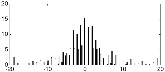
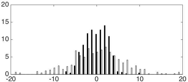
In these histograms, the Y axis indicates how many percent of the images (out of 484) have an error close to the corresponding value along the X axis (as a percentage of the size of the side of the periodic pattern). It can be seen that the distribution errors for a better method are less scattered than for a worse one.
We have proposed a method for searching for periodic patterns on document images, which uses a discrete Fourier transform and showed an average search error in (from the side of the periodic element) on a set of 484 images.
We will describe the details of our application of this method in one of the following articles.
In our previous article on this topic, we talked about the first half of the search problem solution — detection, i.e. determining the presence of periodic elements in the image. Today we will tell how to find the immediate position of the periodic elements in the image, provided that the detection was successful: we are sure that the elements in the image are present. The second part depends heavily on the first, so it is strongly recommended that you first get acquainted with the first, if you have not already done so.
')
Like last time, the Fourier transform will be used for this.
Image model
Like last time, many arguments will be shown for the one-dimensional case, which is then easily transferred to the two-dimensional one.
Recall that
Since we know in advance the structure of the periodic pattern (in the case of the RF passport, the size and period of the holograms), to restore the position of the elements, it is enough to know only the horizontal and vertical shift of the entire template, which is the same as the shift of one of the “eagles”.
Discrete Fourier transform of a shifted periodic pattern
Shift signal pattern
Let's pretend that
Since the phase angle
Phase shift on
The figure shows an example of the DFT phase of a shifted pulsed signal with values
And this is how the amplitude and phase of the DFT looks like for a Gaussian grid like a chessboard:
- DFT -> For a two-dimensional image, the phase shift
Applying again the theorem on the DFT of a shifted signal, one can extend the shift equation and show that the phase angle
As for the one-dimensional case, to obtain a shifted phase
Search for a periodic template
To determine the exact location of the periodic pattern, it is sufficient to estimate its phase shift.
Cutting, scaling and image preprocessing
In the first article, we described the different stages of preprocessing the original image of a passport. First, an area containing a 2x2 grid (similar to a chessboard) and containing 2 patterns horizontally and vertically is cut out of the image. This can be done (with an error of less than 5%), since the physical dimensions of the document, the size and period of the periodic patterns are fixed and known in advance. The position of the region can be set by combining the physical coordinates of the document with its coordinates in the image.
Next, a significant compression and smoothing of the image is performed to suppress the background and to level the differences between the periodic patterns. The figure below shows an image of a cut-out region of a Russian passport, the results of its preprocessing and the amplitude of its DFT.
- processing -> - DFT -> As expected, the DFT amplitude has noticeable peaks with a distribution similar to a chessboard.
Spectrum preprocessing
According to the image model, the original image consists of three independent signals: the background image
After performing the DFT on
To obtain a phase shift
Background Spectrum Suppression
If the background
However, the background image
We have previously mentioned the fact that the DFT positions (frequencies) without peaks do not contain useful information regarding periodic patterns, since they represent the background. Assuming that
The following figure contains a compressed image and an image obtained as a result of the inverse DFT after subtracting the interpolated background spectrum and resetting the DFT at all off-peak frequencies.
- DFT, subtraction of the background spectrum, inverse DFT ----> As expected, only the periodic pattern remained on a plain monotone background, and instances of the periodic pattern became more similar to each other. Note that the background is not black because the DFT value on
Suppressing the spectrum of pattern instances
After removing the background spectrum, we have left
The problem is that the spectrum of the periodic pattern is usually unknown. One of the possible solutions is the experimental calculation of the phase of the presented pattern of the pattern and its subsequent subtraction. In our experiments, we used a different path, assuming that the phase contribution
Phase Shift Recovery
At the end of the spectrum preprocessing, we have the phase angle of the pulsed signal
We can build a system of equations (each equation corresponds to
Or, in matrix form:
The left part of the system contains the “ideal” phase values corresponding to the peaks, and the right part contains the actual value of the DFT phase for this image at the peak positions.
This system is redefined, because she has
Calculation of the initial solution
Let's look at two equations for peaks numbered
This system has 4 valid solutions:
To choose the right solution, we can add to the system the two remaining equations for the peaks
Note that intermediate calculations involving phase angles (difference calculation) are performed in
Finally, the solution
Solution adjustment
The initial solution found above could be good if the remaining spectrum contained only information about
At this stage, the selected solution
Assuming that, in the first approximation of the solution, we were no more mistaken than
So far, we have considered equations for the first 4 peaks.
To use the information about the phase shift contained in the remaining peaks, we can repeat the above process of adjusting the initial solution, replacing
Restoring the location of periodic patterns
Now having a phase shift
The following picture, which you have already seen at the very beginning of the article, presents an example of finding a holographic periodic pattern on a Russian passport.
A box with a circle inside indicates the result found after solving the system of equations. The other boxes indicate the extrapolated positions of the other patterns.
Experimental Results
We used a data set of 484 images of scanned Russian passports with holographic content. For each image in the set, we prepared the true value of the pixel shift of its periodic pattern. The table below contains the experimental results for this data set with the average value of the bias residual as a measure of accuracy.
The error is given as a percentage of the side of a single pattern. The preprocessing consisted of compression to size 56x58 and morphological closure operation; when solving the system for obtaining the phase shift were considered
| Background suppression | Adjustment with OLS | x error | y mistake | General error |
|---|---|---|---|---|
| Missing | Missing | 2.13 | 6.40 | 6.75 |
| Present | Missing | 2.09 | 6.04 | 6.40 |
| Missing | Present | 2.19 | 5.05 | 5.50 |
| Present | Present | 2.20 | 4.77 | 5.25 |
The following figure shows the distribution
In these histograms, the Y axis indicates how many percent of the images (out of 484) have an error close to the corresponding value along the X axis (as a percentage of the size of the side of the periodic pattern). It can be seen that the distribution
Conclusion
We have proposed a method for searching for periodic patterns on document images, which uses a discrete Fourier transform and showed an average search error in
We will describe the details of our application of this method in one of the following articles.
Source: https://habr.com/ru/post/266917/
All Articles