How a relational database works
 Relational databases (DDB) are used everywhere. They come in all sorts of ways, from small and useful SQLite to powerful Teradata. But at the same time there are very few articles explaining the principle of operation and the device of relational databases. Yes, and those that are - quite superficial, without much detail. But in more “fashionable” areas (big data, NoSQL or JS) many more articles are written, and much more profound. Probably, this situation is due to the fact that relational databases are “old” and too boring to be disassembled outside university programs, research papers and books.
In fact, few people really understand how relational databases work. And many developers do not like it when they do not understand something. If relational databases use about 40 years, then there is a reason. RBD is a very interesting thing, because it is based on useful and widely used concepts. If you would like to understand how RBDs work, then this article is for you.
Immediately you need to emphasize: from this material you will not learn how to use the database. However, to assimilate the material, you should be able to write at least a simple connection request and a CRUD request. This is quite enough for understanding the article, the rest will be explained.
The article consists of three parts:
- Overview of low-level and high-level database components.
- Overview of query optimization.
- Overview of transaction and buffer pool management.
')
1. Basics
Once upon a time (in a far-away galaxy), developers had to keep in mind the exact number of operations they code. They felt the algorithms and data structures with all their hearts, because they could not afford to waste processor and memory resources on their slow computers of the past. In this chapter, we will recall some concepts that are necessary for understanding database operation.
1.1. O (1) vs O (n 2 )
Today, many developers do not really think about the time complexity of algorithms ... and they are right! But when you have to work with a large amount of data, or if you need to save milliseconds, the time complexity becomes extremely important.
1.1.1. Concept
The time complexity is used to evaluate the performance of the algorithm, how long the algorithm will be executed for the input data of a certain size. The time complexity is denoted as “O” (read as “O big”). This designation is used in conjunction with a function that describes the number of operations performed by the algorithm for processing input data.
For example, if you say “this algorithm is O large from a certain function”, then this means that for a certain amount of input data, the algorithm needs to perform a number of operations proportional to the value of the function from this certain amount of data.
Here it is not the volume of data that is important, but the dynamics of the increase in the number of operations with increasing volume. The time complexity does not allow to calculate the exact amount, but it is a good way to estimate.
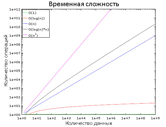
In this graph, you can see how different classes of complexity change. For clarity, a logarithmic scale is used. In other words, the amount of data is rapidly increasing from 1 to 1,000,000. We see that:
- O (1) is “constant time”, that is, its value is constant.
- O (log (n)) - logarithmic time, increases very slowly.
- The worst situation is with the complexity of O (n 2 ) - quadratic time.
- The other two classes of difficulty are rapidly increasing.
1.1.2. Examples
With a small amount of input data, the difference between O (1) and O (n 2 ) is negligible. Suppose we have an algorithm that needs to process 2000 elements.
- The algorithm with O (1) will require 1 operation.
- O (log (n)) - 7 operations.
- O (n) - 2000 operations.
- O (n * log (n)) - 14,000 operations.
- O (n 2 ) - 4,000,000 operations.
It seems that the difference between O (1) and O (n 2 ) is huge, but in fact you will lose no more than 2 ms. Eye blink do not have time, literally. Modern processors perform hundreds of millions of operations per second , and that is why in many projects, developers neglect performance optimization.
But now we take 1 000 000 elements, which is not too much by the standards of the database:
- The algorithm with O (1) for processing will require 1 operation.
- O (log (n)) - 14 operations.
- O (n) - 1,000,000 operations.
- O (n * log (n)) - 14,000,000 operations.
- O (n 2 ) - 1,000,000,000,000 transactions.
In the case of the last two algorithms, you can have time to drink coffee. And if you add another 0 to the number of elements, then during the processing you can take a nap.
1.1.3. Some more details
So that you can navigate:
- Finding an item in a good hash table is O (1).
- In a well-balanced tree - O (log (n)).
- In the array - O (n).
- The best sorting algorithms have O (n * log (n)) complexity.
- Bad sorting algorithms - O (n 2 ).
Below we look at these algorithms and data structures.
There are several time complexity classes:
- Average complexity
- Difficulty at best
- Worst case difficulty
The most common third grade. By the way, the concept of "complexity" is also applicable to the consumption by the algorithm of memory and I / O operations of the disk system.
There are difficulties far worse than n 2 :
- n 4 : characteristic of some bad algorithms.
- 3 n : even worse! Below will be considered one algorithm with a similar time complexity.
- n !: generally hellish trash. You try to wait for the result even on small amounts of data.
- n n : if you have waited for the result of the implementation of this algorithm, then it is time to ask yourself: is it really worth it to you?
1.2. Merge sort
What do you do when you need to sort a collection? Call the sort () function, right? But do you understand how it works?
There are a few good sorting algorithms, but here we look at only one of them: merge sort. Perhaps now this knowledge does not seem useful to you, but you will change your opinion after the chapters on query optimization. Moreover, an understanding of the operation of this algorithm will help to understand the principle of an important operation - merge merging.
1.2.1. Merger
The merge sorting algorithm is based on one trick: to merge two sorted arrays of size N / 2, each requires only N operations, called merge.
Consider an example of a merge operation:
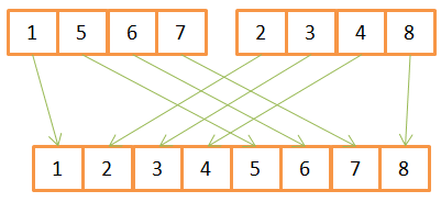
As you can see, to create a sorted array of 8 elements, for each of them you need to carry out one iteration in two source arrays. Since they are already sorted in advance, then:
- First, they compare the available elements
- the smallest of them is transferred to the new array,
- and then returns to the array from which the previous element was taken.
- Steps 1-3 are repeated until only one element remains in one of the source arrays.
- After that, all the remaining elements are transferred from the second array.
This algorithm works well only because both source arrays were sorted in advance, so it does not need to return to their beginning during the next iteration.
An example of merge sort pseudo code:
array mergeSort(array a)
   if(length(a)==1)
      return a[0];
   end if

   //recursive calls
   [left_array right_array] := split_into_2_equally_sized_arrays(a);
   array new_left_array := mergeSort(left_array);
   array new_right_array := mergeSort(right_array);

   //merging the 2 small ordered arrays into a big one
   array result := merge(new_left_array,new_right_array);
   return result;
( « »). , , :
- — .
- — ().
1.2.2.
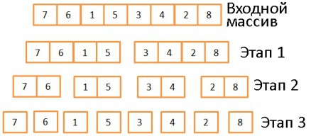
, . , log(N) ( N=8, log(N) = 3). , . 2.
1.2.3.
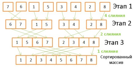
, . 8 :
- 4 , 2 .
- — 2 4 .
- — 1 8 .
log(N), N * log(N).
1.2.4.
?
- , , ( « »).
- , /. , , . , , 100. « ».
- //
- , Hadoop.
! ( ) , . , , .
1.3. , -
, ό . , .
1.3.1.
— . :
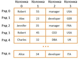
- , — . ( , , ..).
, , - . , , . , , “UK”. N (N — ). , . .
: , (, ). .
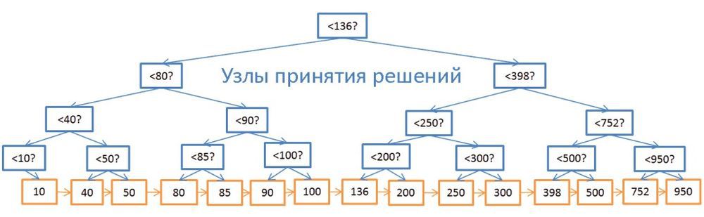
1.3.2.
— , :
- , .
- , .
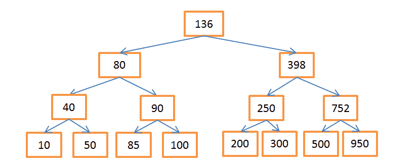
.
N = 15 . , 208:
- , 136. 136 < 208, .
- 398 > 208, , .
- 250 > 208, .
- 200 < 208, . 200 , . , -200 .
, 40:
- -136. 136 > 40, .
- 80 > 40, « ».
- 40 = 40, . ID , ( ), .
- ID , .
. Log(N), .
.
, , . . , “UK”, , , ID , . , log(N) . .
( , , , ..), (.. ). .
+
, , . á (N), . , /, . . — +. , (ID ) («»), .
, . « » , ID . (log(N)) ( ). B- , «» .
, 40 100:
- , 40 , , 40 . .
- , , , 100.
N , . log(N) , . , . + log(N) , N . , + log(N) , . (, 200), N — , , (1 000 000), .
. , , , +, :
- -, .
- , + , á (log(N)), (N).
, + . , + . , «» . : + (log(N)). : . // , , (log(N)) . , .
+ , (, ) MySQL. , InnoDB ( MySQL) .
1.3.3. -
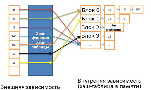
, . - , - (hash join). - ( , ). . - :
- .
- -, . .
- . , .
-:
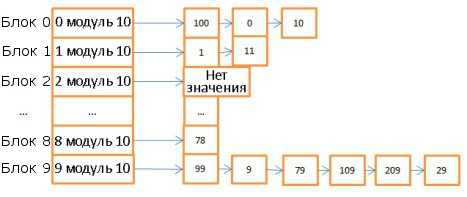
10 , - 10 . : 0, 0, 1, 1, .. .
, 78:
- - , 8.
- 8 .
: .
- 59:
- , 9.
- 9, 99. 99 59, (9), (79), (29).
- .
7 .
, . -, 1 000 000 ( 6 ). 59 , 000059 . -, .
. . -, :
- (, ).
- ( ).
- ( )
..
-, (1).
-
? , :
- - , .
- . , .
- -. , .
Java HashMap, -. Java, .
2.
. .
, . . , , SQLite, . , , SQLite :
- .
- .
:
, , . . , , .
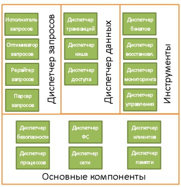
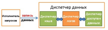
(Core Components):
- . /, . , .
- . , .
- . « » . , .
- . , . , , . , .
- . .
- . .
(Tools):
- . .
- . .
- . .
- . ( ) , , ..
(Query Manager):
- . .
- . .
- .
- . .
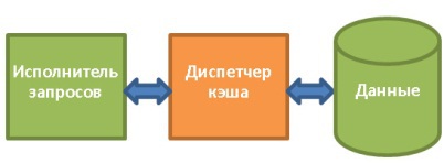
(Data Manager):
- . .
- . .
- . .
, SQL- :
- .
- .
- .
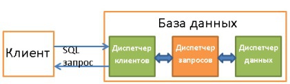
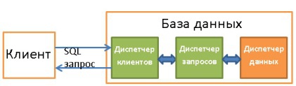
3.
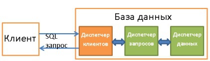
— - /. API (JDBC, ODBC, OLE-DB ..), .
:
- ( ), . DBA.
- , ( ), .
- , .
- , . , , .
- , .
- , .
- - .
4.
. , , . :
- ().
- .
- . .
- .
- .
, :
- Access Path Selection in a Relational Database Management System. 1979 .
- , DB2 9.x .
- , PostgreSQL. .
- SQL . , SQLite . .
- , SQL Server 2005 .
- Oracle 12c.
- “Database System Concepts”: . , /. CS.
- , . /.
4.1.
SQL- . , . , SLECT SELECT.
. , . , WHERE SELECT, .
. :
- .
- .
- . , , substring() ).
, ( ) . DBA.
SQL- ( ). , .
4.2.
:
- .
- .
- .
. , . :
- (). , SQL-.
- . , , .
, :
SELECT PERSON.*
FROM PERSON
WHERE PERSON.person_key IN
(SELECT MAILS.person_key
FROM MAILS
WHERE MAILS.mail LIKE 'christophe%');
:
SELECT PERSON.*
FROM PERSON, MAILS
WHERE PERSON.person_key = MAILS.person_key
and MAILS.mail LIKE 'christophe%';
- . , DISTINCT , UNIQUE, . DISTINCT .
- . , , - , .
- . -, , . , WHERE AGE > 10+2 WHERE AGE > 12. TODATE (- ) .
- Partition pruning. , .
- . , , , , , .
- . ( Oracle), .
- OLAP-. /, , .. , , , OLAP- , .
, .
4.3.
, , . , , .
?
, . , ( 4 8 ). 1 , - . .
. , :
- / .
- :
- .
- (, , ).
- (, , ).
- .
/, .
. , : «» «». , 1 000 «» 1 000 000 — «». — «, », «, »: , , 2-3 .
. . . , , .. . (WHERE AGE=18) (WHERE AGE > 10 AND AGE < 40), , (, ).
. , :
- Oracle: USER/ALL/DBA_TABLES USER/ALL/DBA_TAB_COLUMNS
- DB2: SYSCAT.TABLES SYSCAT.COLUMNS
. , , , 500 , 1 000 000. , , . , . , (, 10%) . , , . .
, . PostgreSQL.
4.4.
CBO (Cost Based Optimization), . , «», «» .
, . ỳ , «» , /. á — , , , if, , ..
:
- .
- ( ) , .
. , , .
4.4.1.
, -. , . , , , (bitmap index). , -. , , .
4.4.2.
, . .
- . . , , .
- . , , WHERE AGE > 20 AND AGE < 40. , AGE.
, á M + log(N), N — , — . . , . - . , - .
- ID . , ό . , :
SELECT LASTNAME, FIRSTNAME from PERSON WHERE AGE = 28
, 28-, ID , .
, :SELECT TYPE_PERSON.CATEGORY from PERSON, TYPE_PERSON WHERE PERSON.AGE = TYPE_PERSON.AGE
TYPE_PERSON PERSON. PERSON, ID .
, /. ID, . - . Oracle. , .
4.4.3.
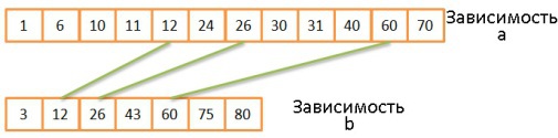
, , , . : . :
- ,
- ,
- (, ).
, -. , A JOIN B , , — .
A JOIN B B JOIN A.
, N , — . , . N M .
- . .
: .
:nested_loop_join(array outer, array inner) for each row a in outer for each row b in inner if (match_join_condition(a,b)) write_result_in_output(a,b) end if end for end for
, á (N*M).
N . N + N*M . , , M + N . , .
ό .
, /.
, , .- , (bunch), .
- , .
- .
, .
:// improved version to reduce the disk I/O. nested_loop_join_v2(file outer, file inner) for each bunch ba in outer // ba is now in memory for each bunch bb in inner // bb is now in memory for each row a in ba for each row b in bb if (match_join_condition(a,b)) write_result_in_output(a,b) end if end for end for end for end for
á , : ( + * ). .
: , , . - -. , .
:- .
- -.
- .
- ( -), .
- .
ό , :- .
- - . .
- .
á :
( / ) * (N / X) + __-() + _- * N
- , á ( + N).
-, /:- - .
- .
- ( , ).
. , . , , . , , .
:- () , .
- .
, , .
, , :- .
- .
- .
. .- .
- , , , .
- , , , .
- 1-3 , .
, á (N + M).
, á O(N * Log(N) + M * Log(M)).
, , -. : , , . . :mergeJoin(relation a, relation b) relation output integer a_key:=0; integer b_key:=0; while (a[a_key]!=null and b[b_key]!=null) if (a[a_key] < b[b_key]) a_key++; else if (a[a_key] > b[b_key]) b_key++; else //Join predicate satisfied write_result_in_output(a[a_key],b[b_key]) //We need to be careful when we increase the pointers integer a_key_temp:=a_key; integer b_key_temp:=b_key; if (a[a_key+1] != b[b_key]) b_key_temp:= b_key + 1; end if if (b[b_key+1] != a[a_key]) a_key_temp:= a_key + 1; end if if (b[b_key+1] == a[a_key] && b[b_key] == a[a_key+1]) a_key_temp:= a_key + 1; b_key_temp:= b_key + 1; end if a_key:= a_key_temp; b_key:= b_key_temp; end if end while
?
, . :
- . , -. , .
- . , , , - . , .
- . -, .
- . , ( ), . , . , ORDER BY/GROUP BY/DISTINCT.
- . .
- . (.1 = .2)? , , (self-join)? .
- . (, , ), -. - .
- /.
DB2, ORACLE SQL Server.
4.4.4.
, , . :
- .
- .
- .
- .
:
SELECT * from PERSON, MOBILES, MAILS,ADRESSES, BANK_ACCOUNTS
WHERE
PERSON.PERSON_ID = MOBILES.PERSON_ID
AND PERSON.PERSON_ID = MAILS.PERSON_ID
AND PERSON.PERSON_ID = ADRESSES.PERSON_ID
AND PERSON.PERSON_ID = BANK_ACCOUNTS.PERSON_ID
. :
- ? (-, , ), 0, 1 2 . , .
- ?
, :
, ?
- -. . . , 34=81 . , (2 * 4)! / (4 + 1)!.. , 34 * (2 * 4)! / (4 + 1)! = 27 216. , 0, 1 2 -, 210 000. , ?
- . , , .
- . , , .
- «» .
:- «», . . , « ».
- . , « , , — -».
. : OUTER JOIN, CROSS JOIN, GROUP BY, ORDER BY, PROJECTION, UNION, INTERSECT, DISTINCT .. .
?
4.4.5. , «»
, . . , .
. . .
, .
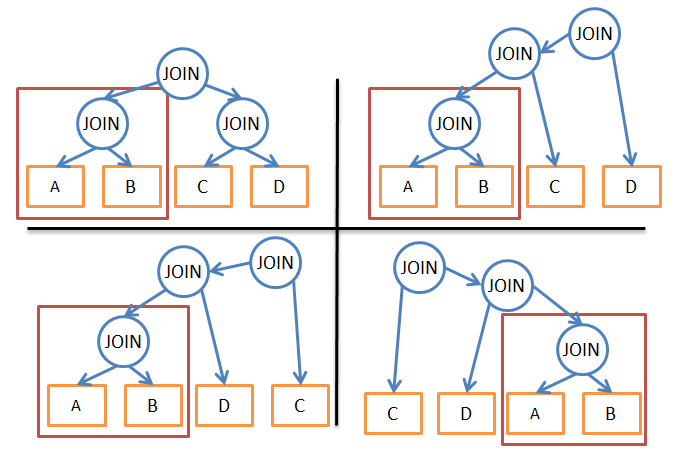
A JOIN B. , , . , , .
ό (2*N)!/(N+1)! « » 3N. 336 81. 8 ( ), 57 657 600 6 561.
, :
procedure findbestplan(S)
if (bestplan[S].cost infinite)
   return bestplan[S]
// else bestplan[S] has not been computed earlier, compute it now
if (S contains only 1 relation)
         set bestplan[S].plan and bestplan[S].cost based on the best way
         of accessing S  /* Using selections on S and indices on S */
     else for each non-empty subset S1 of S such that S1 != S
   P1= findbestplan(S1)
   P2= findbestplan(S - S1)
   A = best algorithm for joining results of P1 and P2
   cost = P1.cost + P2.cost + cost of A
   if cost < bestplan[S].cost
       bestplan[S].cost = cost
      bestplan[S].plan = “execute P1.plan; execute P2.plan;
                 join results of P1 and P2 using A”
return bestplan[S]
, (), :
- - (, ), 3N N*2N.
- (« , , ») .
- « » (, « ») .
, , — .
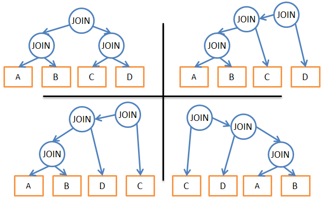
(). . JOIN, JOIN .
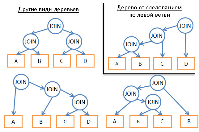
. 4 5 (A, B, C, D E). , . « ».
- , , .
- ( , ).
- , A JOIN B.
- A JOIN B ( ).
- , (A JOIN B) JOIN C.
- .
- …
- : (((A JOIN B) JOIN C) JOIN D) JOIN E)/
, B, C .. , .
« ».
, N*log(N) . á (N*log(N)) (3N) . 20 , 26 3 486 784 401. , ?
. , , . A JOIN B , (A JOIN C) JOIN B , (A JOIN B) JOIN C.
, .
, . .
. - . , , ..
. . , . , , , .
:
- .
- () .
- , .
- , .
- , .
- .
- Y .
- .
, . , , .
, PostgreSQL.
, (Simulated Annealing), (Iterative Improvement), (Two-Phase Optimization). , , , — .
4.4.6.
, .
. , SQLite. «» , :
- SQLite CROSS JOIN.
- .
- , .
- 3.8.0 « » (Nearest Neighor). 3.8.0 «N » (N3, N Nearest Neighbors).
. IBM DB2, , 7 :
- :
- 0 — . , .
- 1 —
- 2 —
- :
- 3 —
- 5 — ,
- 7 — ,
- 9 — , . , .
5. :
- , .
- , ). , , .
- :
- .
- .
- , ( ), AND .
, , , — . , , .
(GROUP BY, DISTINCT ..) .
4.4.7.
, . . , . , , , , .
. , , . , (JOIN, SORT BY ..) , , . .
5.
. , :
- . , - /.
- — . , .
5.1.
, . .
, , . , . , , :
- ( ) ( ID ).
- .
, : «» , SSD, RAID . , 100-100 000 , .
. , . .
5.1.1.
, , , , .
, . , , .
. (, latch), .
, , . (speculative prefetching) (, 1, 3, 5, 7, 9, 11) (sequential prefetching) ( .
« /» (buffer/cache hit ratio). , , . . Oracle.
, . . . , . .
5.1.2.
( , SQL Server, MySQL, Oracle DB2) LRU (Least Recently Used). , , , .
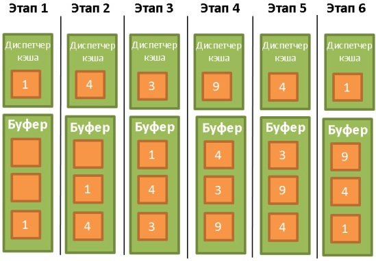
, (latch), . :
- 1 .
- 4 .
- 3.
- 9. - . 1, . 9.
- 4. , .
- 1. , 3, .
, . ? , / ? , , , .
, . Oracle:
« , , . , . , LRU, ».
LRU — LRU-K. SQL Server LRU-K = 2. , , . , , . . , , , . , , - . , .
, SQL Server LRU-K 2. . 1993- .
, LRU-K . 2Q CLOCK ( LRU-K), MRU (Most Recently Used, LRU, , LRFU (Least Recently and Frequently Used) .. , .
5.1.3.
, , , . /.
, ( ), . «», , . , . .
5.2.
, . , ACID-.
5.2.1. « » ( , )
ACID- (Atomicity, Isolation, Durability, Consistency) — , , 4 :
- (Atomicity). «» , . 10 . «», .
- (Isolation). , , , .
- (Durability). (commited), , (, ).
- () (Consistency). ( ). .

- SQL- , , . , . — . , :
- 1 $100 .
- 2 $50 .
ACID-:
- , 1 ( , ), , $100 , ( « »).
- , 1 2 , $100 . .
- , 1 , 1.
- .
, .
, . SQL 4 :
- (Serializable). . SQLite. , .
- (Repeatable read). MySQL. , : , , . , . .
,SELECT count(1) from TABLE_X
. count(1), .
. - (Read commited). Oracle, PostgreSQL SQL Server. , , . , ; , . , ( ), .
(non-repeatable read). - (Read uncommited). . . , ; ( , ). , . , , .
.
(, , PostgreSQL, Oracle SQL Server). , .
. .
5.2.2.
, , , (, ).
, , .
, , . , , .
.
. ( ), .
( ):
- .
- - / , , .
- . .
- , .
, . , . . , .
5.2.3.
(locks) / .
- , . , , .
.
, . ? . , . . - , , . . , .
— , . - ( ). , .
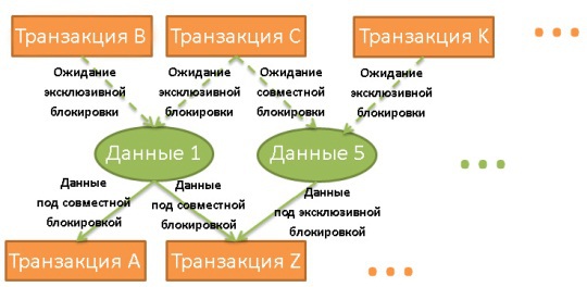
(deadlock)
, :
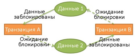
1 2. 2 1.
, ( ). :
- , ( , )?
- , ?
- , ?
- ?
, , .
- , . , . ( , , ), : . , .
, . , . .
, . , , . , .
DB2 SQL Server , :
- (growing phase), , .
- (shrinking phase), ( , ), .
, :
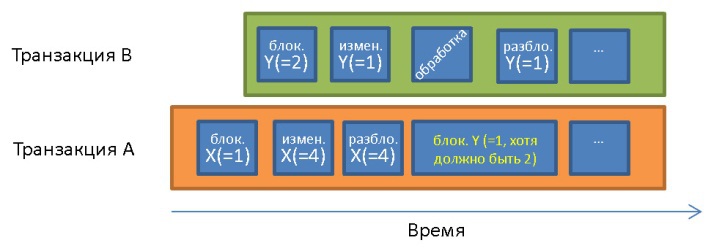
X = 1 Y = 1. Y = 1, . Y = 2.
, :
- , , .
- , , . .
, , , . , . , .
, , ( , , , , ), .
— .
- .
- () .
- , , , (, , ).
, :
- , .
- .
, , , , . .
— — , , ( ). , PostgreSQL.
(DB2 9.7, SQL Server) . , PostgreSQL, MySQL Oracle, .
: . , , ..
, , , . .
, : MySQL, PostgreSQL, Oracle.
5.2.4.
, . , . .
, , , .
, , .
:
- /. ( ), . . , , «» .
- . . . , .
WAL
/ . . .
( , Oracle, SQL Server, DB2, PostgreSQL, MySQL SQLite) WAL (Write-Ahead Logging). :
- , , .
- .
- , .
. . , , . ?
! , , , « ». , , , . , .
ARIES
1992 IBM WAL, ARIES. ARIES . , .
, ARIES Algorithms for Recovery and Isolation Exploiting Semantics. :
- .
- .
, :
- .
- .
- . , UNIQUE, .
- .
, , .
? , , .
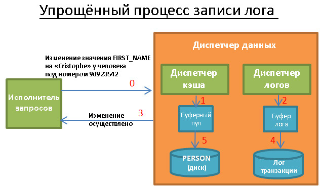
(//) . :
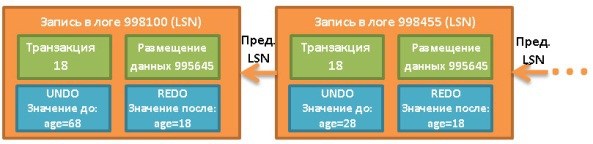
- LSN (Log Sequence Number). , . , LSN LSN . LSN , .
- TransID. , .
- PageID. , .
- PrevLSN. , .
- UNDO. .
, , UNDO / ( UNDO) , ( UNDO). ARIES , . - REDO. .
, ( , ) LSN , .
, UNDO PostgreSQL. , . .
, , UPDATE FROM PERSON SET AGE = 18;. 18:
LSN. , ( ).
, .
:
- .
- .
- , , , , .
- . .
- . .
, , 1 5. , « - ». , , .
STEAL FORCE
5 , REDO. « NO-FORCE».
FORCE . 5 .
, ( STEAL) , , (NO-STEAL). , : ?
:
- STEAL/NO-FORCE UNDO REDO. , ( ARES). .
- STEAL/FORCE UNDO.
- NO-STEAL/NO-FORCE — REDO.
- NO-STEAL/FORCE . , .
, ? , ( №1: !). .
ARIES :
- . , , . , . . , .
- . REDO. . LSN , , .
LSN(__)>=LSN(__), . , . , .
LSN(__)<LSN(__), .
, , . . - . . UNDO PrevLSN.
, . , . , , . ARIES , .
«», , - , . REDO UNDO , :
- ( ).
- ( , ).
, . , .
. ARIES . , LSN. , LSN.
6.
Architecture of a Database System. , .
, , . :
- .
- , .
- .
- .
, NoSQL . , NoSQL- . , .
, - , , , , :

.
Source: https://habr.com/ru/post/266811/
All Articles