Why do I need AshleyMadison if I don't smoke?
As you all probably already know, recently dumps of AshleyMadison bases were posted. I decided not to miss the opportunity and analyze the real data of the dating platform. Let's try to predict the client's solvency according to its characteristics such as age, height, weight, habits, etc.

Let's try?
In this example, I will use iPython notebook. For those who are engaged in analyzing data in Python and have not yet used iPython notebook - I highly recommend it!
')
To build the model we will use anonymized data.
1. Data preparation in MySQL
To begin, fill in the dumps in MySQL and delete all users with id <35,000,000 for ease of further processing. I took the member_details and aminno_member tables.
Data uploading is not very fast, even on a server with SSD (some tables weigh about 10 Gigov)
Next, we need to fill in the payment data from csv and get the amount for each user. As a result, the table turned out to be pays with id and sum fields.
2. Load data into pandas
Join 3 tables by user id and get DataFrame for further processing. We take only users with photos, I think that this is a sign of at least some activity in the system:
Extract the year and month of birth:
Let us try to analyze whether the target variable (paid / not paid) depends on the user's characteristics? Does it make sense to build a model?
We divide the analyzed users into 2 parts: df0 - those who paid at least some, df1 - did not pay anything.
We build 2 histograms for each user parameter. Red - those who paid in blue - not paid.
Consider the most interesting:
Year of birth:
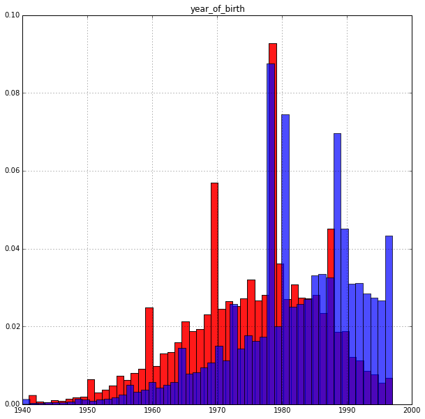
The result is quite expected: age affects the target variable. Older pay more willingly. The peak of the histogram in paying accounts for about 35 years.
Weight:
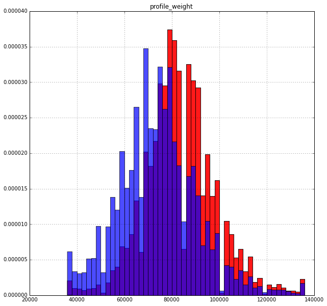
It is more interesting here: those who weigh more are more willing to pay. Although it is also quite logical
Growth:
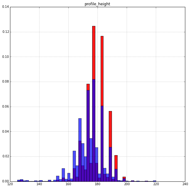
High pay a little more willing. The distribution is very uneven. Perhaps the growth on the site is not a number, but an interval.
Smoking:
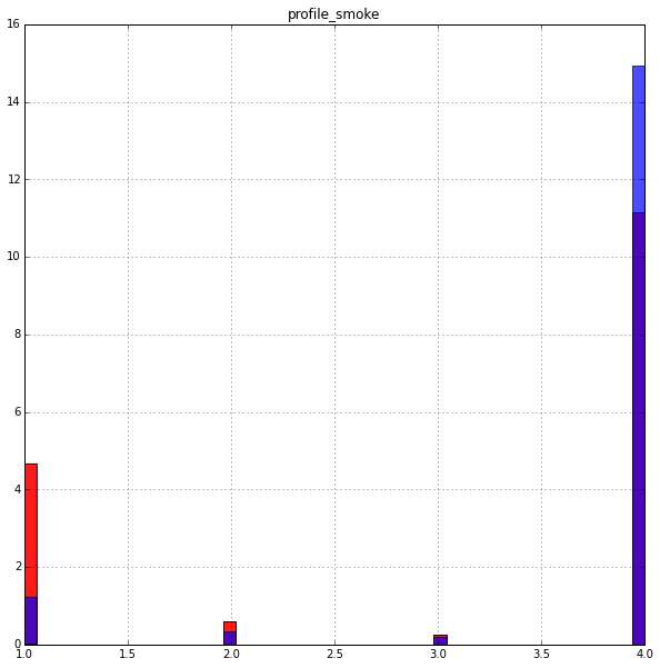
To the question of the title of the article. The obvious dependence is viewed, the question is - what do the values 1,2,3,4 mean?
The remaining user settings do not give such an interesting picture, although they also have their own contribution. There is a complete version of this notebook where you can see all histograms.
2. The prediction of the probability of payment
First, select the target variable (paid / not paid) which we will predict:
We single out the categorical signs and binarize them:
Select the metric signs and combine them with the result of binarization:
We divide the sample into 2 parts 90% and 10%. At first we will train and tyunit model. On the second - to assess the accuracy of the resulting model.
We train the RandomForest classifier and select the optimal parameters.
We estimate the significance of the signs:
The most significant (by decreasing significance): year_of_birth, profile_weight, profile_height.
Assess the quality of the model on the test sample and build a ROC curve:
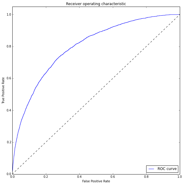
To measure the quality of the classifier we will use the ROC_AUC score
ROC_AUC = 0.79926
results
Predict the propensity of users to pay for services is really possible. Accuracy is not very high (roc_auc = 0.8), but we used only a part of the parameters and did not pay attention to behavioral factors at all (no data).
What's next?
UPD:
For those who want to play with the data, I post a dump of the DataFrame myself
yadi.sk/d/YaNM8DTZj2ybn
And go!
Let's try?
In this example, I will use iPython notebook. For those who are engaged in analyzing data in Python and have not yet used iPython notebook - I highly recommend it!
')
To build the model we will use anonymized data.
1. Data preparation in MySQL
To begin, fill in the dumps in MySQL and delete all users with id <35,000,000 for ease of further processing. I took the member_details and aminno_member tables.
Data uploading is not very fast, even on a server with SSD (some tables weigh about 10 Gigov)
Next, we need to fill in the payment data from csv and get the amount for each user. As a result, the table turned out to be pays with id and sum fields.
2. Load data into pandas
Join 3 tables by user id and get DataFrame for further processing. We take only users with photos, I think that this is a sign of at least some activity in the system:
engine = create_engine('mysql://login:pass@localhost:3306/db') # Creating MySQL engine sql = """ SELECT md.pnum, p.sum, am.gender, am.photos_public, md.profile_weight, md.profile_height, md.eye_color, md.hair_color, md.dob, md.profile_smoke, md.profile_ethnicity, md.profile_bodytype, md.profile_initially_seeking FROM `member_details` AS md JOIN `aminno_member` AS am ON md.pnum = am.pnum LEFT JOIN pays AS p ON md.pnum = p.id WHERE md.dob is not null AND (am.photos_public > 0 OR p.sum is not NULL) """ df = pd.read_sql_query(sql, engine).fillna(0).set_index('pnum') #Reading data from mysql DB to pandas dataframe Extract the year and month of birth:
df['month_of_birth'] = df['dob'].apply(lambda x:x.month) df['year_of_birth'] = df['dob'].apply(lambda x:x.year) Let us try to analyze whether the target variable (paid / not paid) depends on the user's characteristics? Does it make sense to build a model?
We divide the analyzed users into 2 parts: df0 - those who paid at least some, df1 - did not pay anything.
THRESHOLD = 0.0001 df0 = df[(df['sum'] > THRESHOLD)] df1 = df[(df['sum'] < THRESHOLD)] We build 2 histograms for each user parameter. Red - those who paid in blue - not paid.
cols = ['profile_weight','profile_height','year_of_birth','month_of_birth', 'eye_color', 'hair_color','profile_smoke', 'profile_ethnicity', 'profile_bodytype', 'profile_initially_seeking','gender'] for col in cols: plt.figure(figsize=(10,10)) df0[col].hist(bins=50, alpha=0.9, color = 'red', normed=1) df1[col].hist(bins=50, alpha=0.7, normed=1) plt.title(col) plt.show() Consider the most interesting:
Year of birth:
The result is quite expected: age affects the target variable. Older pay more willingly. The peak of the histogram in paying accounts for about 35 years.
Weight:
It is more interesting here: those who weigh more are more willing to pay. Although it is also quite logical
Growth:
High pay a little more willing. The distribution is very uneven. Perhaps the growth on the site is not a number, but an interval.
Smoking:
To the question of the title of the article. The obvious dependence is viewed, the question is - what do the values 1,2,3,4 mean?
The remaining user settings do not give such an interesting picture, although they also have their own contribution. There is a complete version of this notebook where you can see all histograms.
2. The prediction of the probability of payment
First, select the target variable (paid / not paid) which we will predict:
y = (df['sum'] > THRESHOLD).astype(np.int32) We single out the categorical signs and binarize them:
categorical = ['month_of_birth', 'eye_color', 'hair_color','profile_smoke', 'profile_ethnicity', 'profile_bodytype', 'profile_initially_seeking'] ohe = preprocessing.OneHotEncoder(dtype=np.float32) Xcategories = ohe.fit_transform(df[categorical]).todense() Select the metric signs and combine them with the result of binarization:
numeric = ['gender','profile_weight','profile_height','year_of_birth'] Xnumeric = df[numeric].as_matrix() X = np.hstack((Xcategories,Xnumeric)) We divide the sample into 2 parts 90% and 10%. At first we will train and tyunit model. On the second - to assess the accuracy of the resulting model.
X_train, X_test, y_train, y_test = cross_validation.train_test_split(X, y, test_size=0.1, random_state=7) We train the RandomForest classifier and select the optimal parameters.
from sklearn.preprocessing import StandardScaler from sklearn.ensemble import RandomForestClassifier from sklearn import decomposition, pipeline, metrics, grid_search rf = RandomForestClassifier(random_state=7, n_jobs=4) scl = StandardScaler() clf = pipeline.Pipeline([('scl', scl), ('rf', rf)]) param_grid = {'rf__n_estimators': (100,200), 'rf__max_depth': (10,20), } model = grid_search.GridSearchCV(estimator = clf, param_grid=param_grid, scoring='roc_auc', verbose=10, cv=3) model.fit(X_train, y_train) print("Best score: %0.3f" % model.best_score_) print("Best parameters set:") best_parameters = model.best_estimator_.get_params() for param_name in sorted(param_grid.keys()): print("\t%s: %r" % (param_name, best_parameters[param_name])) Best score: 0.802 Best parameters set: rf__max_depth: 20 rf__n_estimators: 200 We estimate the significance of the signs:
best = model.best_estimator_ print best.steps[1][1].feature_importances_ [ 0.01083346 0.00745737 0.00754652 0.00764087 0.0075468 0.00769951 0.00780227 0.0076059 0.00747405 0.00733789 0.00720822 0.00720196 0.01067164 0.00229657 0.00271315 0.00403617 0.00453246 0.00420906 0.01227852 0.00166965 0.00060406 0.00293115 0.00347255 0.00581456 0.00176878 0.00060611 0.00129565 0.06303697 0.00526695 0.00408359 0.04618295 0.03014204 0.00401634 0.00312768 0.0041792 0.00073294 0.00260749 0.00137382 0.00385419 0.03020433 0.00788376 0.01423438 0.00953692 0.01218361 0.00685376 0.00812187 0.00433835 0.00294894 0.01210143 0.00806778 0.00458055 0.01323813 0.01434638 0.0120177 0.03383968 0.1623351 0.11347244 0.2088358 ] The most significant (by decreasing significance): year_of_birth, profile_weight, profile_height.
Assess the quality of the model on the test sample and build a ROC curve:
from sklearn.metrics import roc_curve,roc_auc_score y_pred = best.predict_proba(X_test).T[1] print roc_auc_score(y_test, y_pred) fpr, tpr , thresholds = roc_curve(y_test, y_pred) plt.figure(figsize=(10,10)) plt.plot(fpr, tpr, label='ROC curve') plt.plot([0, 1], [0, 1], 'k--') plt.xlim([0.0, 1.0]) plt.ylim([0.0, 1.05]) plt.xlabel('False Positive Rate') plt.ylabel('True Positive Rate') plt.title('Receiver operating characteristic') plt.legend(loc="lower right") plt.show() To measure the quality of the classifier we will use the ROC_AUC score
ROC_AUC = 0.79926
results
Predict the propensity of users to pay for services is really possible. Accuracy is not very high (roc_auc = 0.8), but we used only a part of the parameters and did not pay attention to behavioral factors at all (no data).
What's next?
- You can try to predict something based on tastes / preferences. The database has the fields 'pref_opento', 'pref_lookingfor' of the form "12 | 17 | 58 | 97" - these are links to some directory which is not. You can build a model without it, but you will not be able to interpret it.
- Try a regression model and predict the amount, not the fact of payment.
- Play around with algorithms, sample size, sample parameters (I used photos_public> 0)
- Your suggestions?
UPD:
For those who want to play with the data, I post a dump of the DataFrame myself
yadi.sk/d/YaNM8DTZj2ybn
import joblib import pandas as pd df = joblib.load("1.pkl") print df And go!
Source: https://habr.com/ru/post/266639/
All Articles