How a month to get a lot of pumping in Data Science
Hi, Habr!

My name is Gleb , I have been working in retail analytics for a long time and now I am engaged in using machine learning in this field. Not long ago, I met the guys from MLClass.ru , who in a very short time rather strongly pumped me into the field of Data Science . Thanks to them, literally in a month I began actively submitting to kaggle. Therefore, this series of publications will describe my experience in studying Data Science: all the mistakes that were made, as well as valuable advice that the guys gave me. Today I will talk about the experience of participating in The Analytics Edge (Spring 2015) . This is my first article - do not judge strictly.
The described competition was held as part of the “The Analytics Edge” course from the “Massachusetts Institute of Technology” . Below I will provide the code in the R language, which can be found entirely here .
')
Any seller would like to know what characteristics of the product increase the likelihood of the sale of goods. In this competition, it was proposed to investigate models that would predict the likelihood of selling an Apple iPad on a database obtained from the eBay website.
The data proposed for study consisted of two files:
To begin with we will connect the libraries applied in work.
Now load the data.
Let's look at the data structure.
The data set consists of 11 variables:
Thus, we have three types of variables: textual description , numerical startprice, and all the others are factorial.
Let's see which part of the goods has a description
Since not all products have a description, I assumed that this parameter may affect the probability of sale. To take this into account, we will create a variable that will take the value 1 , if the description is, and 0 , in the opposite case.
Based on the text description, we will create variables for the model by highlighting common words. For this we use the tm library.
Now we will bring the remaining text variables to the data type factor to prevent them from being treated as text by the model. And combine them with the variables derived from the product description. For this we use a very convenient library magnittr
Let's look at the resulting set of variables.
Perform the normalization of the startprice variable so that this variable does not exert undue influence on the model results, due to its much wider range compared to other variables.
With the obtained data set we will create models. To assess the accuracy of the assessment of models, we will apply the same assessment that was chosen in the competition. This is AUC . This parameter is often used to evaluate classification models. It reflects the probability with which the model will correctly determine the dependent variable from a random data set. An ideal model will show an AUC value of 1.0, and a model with an equally probable random guessing - 0.5 .
Since the format of the competition involves a limited number of times per day, which can be verified by the resulting model by uploading the results to the site, then to evaluate the models, we will separate our own test sample from the training data set. To obtain a balanced sample, use the caTools library.
Create a logistic regression model
Let's look at the significance of variables for the model.
It can be seen that for a simple logistic model there are few significant variables in the data
We estimate the AUC on the test data. For this we use the library ROCR
The result obtained using this model is already very good, but it is necessary to compare it with the estimates of other models.
Now look at the results obtained using the CART model.
The model makes the assessment worse than the previous one. Let's try to improve the results using the selection of parameters by cross-validation . We will select the parameter cp , which determines the complexity of the model
Insert the proposed value and evaluate the resulting model.
Let's look at the results of the most difficult model in theory, but very simple to use - Random Forest
As you can see, the model already shows the best results of all used. Let's try to improve it by eliminating unnecessary variables. The presence of a built-in assessment of the importance of variables in the model will help us.
On the left graph, we see that there is a feature that does not improve the quality of the model. Remove it and evaluate the resulting model.
The assessment showed that there was no improvement in the model, but, based on common sense, I believe that having the word excel in the product description is unlikely to affect sales, and simplifying the model (without significant damage to quality) improves its interpretation.
Thus, the best results from all the models studied were logistic regression. As a result, on the Public Board (50% estimate of all available test data), the model with a score of 0.84724 ranked 211 out of 1884, but dropped to 1291 in the final protocol.
Next time I plan to talk about how the quality of the model is influenced by the size of the training sample using the example of the Digit Recognizer task, and the application of the principal component method in the same task. Then I will talk about the experience of participating in the Bag of Words Meets Bags of Popcorn competition, as well as a long study in the well-known task Titanic: Machine Learning from Disaster , in which I will tell you about how knowledge about Titanic and the catastrophe help solve the problem.
And finally, I recommend to sign up for the guys on the course on data analysis . In my experience:
See you!
My name is Gleb , I have been working in retail analytics for a long time and now I am engaged in using machine learning in this field. Not long ago, I met the guys from MLClass.ru , who in a very short time rather strongly pumped me into the field of Data Science . Thanks to them, literally in a month I began actively submitting to kaggle. Therefore, this series of publications will describe my experience in studying Data Science: all the mistakes that were made, as well as valuable advice that the guys gave me. Today I will talk about the experience of participating in The Analytics Edge (Spring 2015) . This is my first article - do not judge strictly.
The described competition was held as part of the “The Analytics Edge” course from the “Massachusetts Institute of Technology” . Below I will provide the code in the R language, which can be found entirely here .
')
Task Description
Any seller would like to know what characteristics of the product increase the likelihood of the sale of goods. In this competition, it was proposed to investigate models that would predict the likelihood of selling an Apple iPad on a database obtained from the eBay website.
Data
The data proposed for study consisted of two files:
- eBayiPadTrain.csv - a data set for creating a model. Contains 1861 products.
- eBayiPadTest.csv - data for model evaluation
To begin with we will connect the libraries applied in work.
library(dplyr) # library(readr) # Now load the data.
eBayTrain <- read_csv("eBayiPadTrain.csv") eBayTest <- read_csv("eBayiPadTest.csv") Let's look at the data structure.
summary(eBayTrain) ## description biddable startprice condition ## Length:1861 Min. :0.0000 Min. : 0.01 Length:1861 ## Class :character 1st Qu.:0.0000 1st Qu.: 80.00 Class :character ## Mode :character Median :0.0000 Median :179.99 Mode :character ## Mean :0.4498 Mean :211.18 ## 3rd Qu.:1.0000 3rd Qu.:300.00 ## Max. :1.0000 Max. :999.00 ## cellular carrier color ## Length:1861 Length:1861 Length:1861 ## Class :character Class :character Class :character ## Mode :character Mode :character Mode :character ## ## ## ## storage productline sold UniqueID ## Length:1861 Length:1861 Min. :0.0000 Min. :10001 ## Class :character Class :character 1st Qu.:0.0000 1st Qu.:10466 ## Mode :character Mode :character Median :0.0000 Median :10931 ## Mean :0.4621 Mean :10931 ## 3rd Qu.:1.0000 3rd Qu.:11396 ## Max. :1.0000 Max. :11861 str(eBayTrain) ## Classes 'tbl_df', 'tbl' and 'data.frame': 1861 obs. of 11 variables: ## $ description: chr "iPad is in 8.5+ out of 10 cosmetic condition!" "Previously used, please read description. May show signs of use such as scratches to the screen and " "" "" ... ## $ biddable : int 0 1 0 0 0 1 1 0 1 1 ... ## $ startprice : num 159.99 0.99 199.99 235 199.99 ... ## $ condition : chr "Used" "Used" "Used" "New other (see details)" ... ## $ cellular : chr "0" "1" "0" "0" ... ## $ carrier : chr "None" "Verizon" "None" "None" ... ## $ color : chr "Black" "Unknown" "White" "Unknown" ... ## $ storage : chr "16" "16" "16" "16" ... ## $ productline: chr "iPad 2" "iPad 2" "iPad 4" "iPad mini 2" ... ## $ sold : int 0 1 1 0 0 1 1 0 1 1 ... ## $ UniqueID : int 10001 10002 10003 10004 10005 10006 10007 10008 10009 10010 ... The data set consists of 11 variables:
- description - text description of the product provided by the seller
- biddable - the item has been auctioned (= 1) or at a fixed price (= 0)
- startprice - starting price for the auction (if biddable = 1) or selling price (if biddable = 0)
- condition - the condition of the goods (new, used, etc.)
- cellular - a product with a mobile connection (= 1) or not (= 0)
- carrier - carrier (if cellular = 1)
- color - color
- storage - memory size
- productline - product model name
- sold - whether the item was sold (= 1) or not (= 0). This will be the dependent variable.
- UniqueID - unique sequence number
Thus, we have three types of variables: textual description , numerical startprice, and all the others are factorial.
Creating additional variables
Let's see which part of the goods has a description
table(eBayTrain$description == "") ## ## FALSE TRUE ## 790 1071 Since not all products have a description, I assumed that this parameter may affect the probability of sale. To take this into account, we will create a variable that will take the value 1 , if the description is, and 0 , in the opposite case.
eBayTrain$is_descr = as.factor(eBayTrain$description == "") table(eBayTrain$description == "", eBayTrain$is_descr) ## ## FALSE TRUE ## FALSE 790 0 ## TRUE 0 1071 Creating variables for a model from a text description
Based on the text description, we will create variables for the model by highlighting common words. For this we use the tm library.
library(tm) ## ## Loading required package: NLP ## , CorpusDescription <- Corpus(VectorSource(c(eBayTrain$description, eBayTest$description))) ## CorpusDescription <- tm_map(CorpusDescription, content_transformer(tolower)) CorpusDescription <- tm_map(CorpusDescription, PlainTextDocument) ## CorpusDescription <- tm_map(CorpusDescription, removePunctuation) ## -, .. , CorpusDescription <- tm_map(CorpusDescription, removeWords, stopwords("english")) ## , .. CorpusDescription <- tm_map(CorpusDescription, stemDocument) ## dtm <- DocumentTermMatrix(CorpusDescription) ## sparse <- removeSparseTerms(dtm, 0.97) ## data.frame DescriptionWords = as.data.frame(as.matrix(sparse)) colnames(DescriptionWords) = make.names(colnames(DescriptionWords)) DescriptionWordsTrain = head(DescriptionWords, nrow(eBayTrain)) DescriptionWordsTest = tail(DescriptionWords, nrow(eBayTest)) Now we will bring the remaining text variables to the data type factor to prevent them from being treated as text by the model. And combine them with the variables derived from the product description. For this we use a very convenient library magnittr
library(magrittr) eBayTrain %<>% mutate(condition = as.factor(condition), cellular = as.factor(cellular), carrier = as.factor(carrier), color = as.factor(color), storage = as.factor(storage), productline = as.factor(productline), sold = as.factor(sold)) %>% select(-description, -UniqueID ) %>% cbind(., DescriptionWordsTrain) Let's look at the resulting set of variables.
str(eBayTrain) ## 'data.frame': 1861 obs. of 30 variables: ## $ biddable : int 0 1 0 0 0 1 1 0 1 1 ... ## $ startprice : num 159.99 0.99 199.99 235 199.99 ... ## $ condition : Factor w/ 6 levels "For parts or not working",..: 6 6 6 4 5 6 3 3 6 6 ... ## $ cellular : Factor w/ 3 levels "0","1","Unknown": 1 2 1 1 3 2 1 1 2 1 ... ## $ carrier : Factor w/ 7 levels "AT&T","None",..: 2 7 2 2 6 1 2 2 6 2 ... ## $ color : Factor w/ 5 levels "Black","Gold",..: 1 4 5 4 4 3 3 5 5 5 ... ## $ storage : Factor w/ 5 levels "128","16","32",..: 2 2 2 2 5 3 2 2 4 3 ... ## $ productline: Factor w/ 12 levels "iPad 1","iPad 2",..: 2 2 4 9 12 9 8 10 1 4 ... ## $ sold : Factor w/ 2 levels "0","1": 1 2 2 1 1 2 2 1 2 2 ... ## $ is_descr : Factor w/ 2 levels "FALSE","TRUE": 1 1 2 2 1 2 2 2 2 2 ... ## $ box : num 0 0 0 0 0 0 0 0 0 0 ... ## $ condit : num 1 0 0 0 0 0 0 0 0 0 ... ## $ cosmet : num 1 0 0 0 0 0 0 0 0 0 ... ## $ devic : num 0 0 0 0 0 0 0 0 0 0 ... ## $ excel : num 0 0 0 0 0 0 0 0 0 0 ... ## $ fulli : num 0 0 0 0 0 0 0 0 0 0 ... ## $ function. : num 0 0 0 0 0 0 0 0 0 0 ... ## $ good : num 0 0 0 0 0 0 0 0 0 0 ... ## $ great : num 0 0 0 0 0 0 0 0 0 0 ... ## $ includ : num 0 0 0 0 0 0 0 0 0 0 ... ## $ ipad : num 1 0 0 0 0 0 0 0 0 0 ... ## $ item : num 0 0 0 0 0 0 0 0 0 0 ... ## $ light : num 0 0 0 0 0 0 0 0 0 0 ... ## $ minor : num 0 0 0 0 0 0 0 0 0 0 ... ## $ new : num 0 0 0 0 0 0 0 0 0 0 ... ## $ scratch : num 0 1 0 0 0 0 0 0 0 0 ... ## $ screen : num 0 1 0 0 0 0 0 0 0 0 ... ## $ use : num 0 2 0 0 0 0 0 0 0 0 ... ## $ wear : num 0 0 0 0 0 0 0 0 0 0 ... ## $ work : num 0 0 0 0 0 0 0 0 0 0 ... Perform the normalization of the startprice variable so that this variable does not exert undue influence on the model results, due to its much wider range compared to other variables.
eBayTrain$startprice <- (eBayTrain$startprice - mean(eBayTrain$startprice))/sd(eBayTrain$startprice) Models
With the obtained data set we will create models. To assess the accuracy of the assessment of models, we will apply the same assessment that was chosen in the competition. This is AUC . This parameter is often used to evaluate classification models. It reflects the probability with which the model will correctly determine the dependent variable from a random data set. An ideal model will show an AUC value of 1.0, and a model with an equally probable random guessing - 0.5 .
Since the format of the competition involves a limited number of times per day, which can be verified by the resulting model by uploading the results to the site, then to evaluate the models, we will separate our own test sample from the training data set. To obtain a balanced sample, use the caTools library.
set.seed(1000) ## library(caTools) split <- sample.split(eBayTrain$sold, SplitRatio = 0.7) train <- filter(eBayTrain, split == T) test <- filter(eBayTrain, split == F) Logistic classification
Create a logistic regression model
model_glm1 <- glm(sold ~ ., data = train, family = binomial) Let's look at the significance of variables for the model.
summary(model_glm1) ## ## Call: ## glm(formula = sold ~ ., family = binomial, data = train) ## ## Deviance Residuals: ## Min 1Q Median 3Q Max ## -2.6620 -0.7308 -0.2450 0.6229 3.5600 ## ## Coefficients: ## Estimate Std. Error z value Pr(>|z|) ## (Intercept) 11.91318 619.41930 0.019 0.984655 ## biddable 1.52257 0.16942 8.987 < 2e-16 ## startprice -1.96460 0.19122 -10.274 < 2e-16 ## conditionManufacturer refurbished 0.92765 0.59405 1.562 0.118394 ## conditionNew 0.64792 0.38449 1.685 0.091964 ## conditionNew other (see details) 0.98380 0.50308 1.956 0.050517 ## conditionSeller refurbished -0.03144 0.40675 -0.077 0.938388 ## conditionUsed 0.43817 0.27167 1.613 0.106767 ## cellular1 -13.13755 619.41893 -0.021 0.983079 ## cellularUnknown -13.50679 619.41886 -0.022 0.982603 ## carrierNone -13.25989 619.41897 -0.021 0.982921 ## carrierOther 12.51777 622.28887 0.020 0.983951 ## carrierSprint 0.88998 0.69925 1.273 0.203098 ## carrierT-Mobile 0.02578 0.89321 0.029 0.976973 ## carrierUnknown -0.43898 0.41684 -1.053 0.292296 ## carrierVerizon 0.15653 0.36337 0.431 0.666625 ## colorGold 0.10763 0.53565 0.201 0.840755 ## colorSpace Gray -0.13043 0.30662 -0.425 0.670564 ## colorUnknown -0.14471 0.20833 -0.695 0.487307 ## colorWhite -0.03924 0.22997 -0.171 0.864523 ## storage16 -1.09720 0.50539 -2.171 0.029933 ## storage32 -1.14454 0.51860 -2.207 0.027315 ## storage64 -0.50647 0.50351 -1.006 0.314474 ## storageUnknown -0.29305 0.63389 -0.462 0.643867 ## productlineiPad 2 0.33364 0.28457 1.172 0.241026 ## productlineiPad 3 0.71895 0.34595 2.078 0.037694 ## productlineiPad 4 0.81952 0.36513 2.244 0.024801 ## productlineiPad 5 2.89336 1080.03688 0.003 0.997863 ## productlineiPad Air 2.15206 0.40290 5.341 9.22e-08 ## productlineiPad Air 2 3.05284 0.50834 6.005 1.91e-09 ## productlineiPad mini 0.40681 0.30583 1.330 0.183456 ## productlineiPad mini 2 1.59080 0.41737 3.811 0.000138 ## productlineiPad mini 3 2.19095 0.53456 4.099 4.16e-05 ## productlineiPad mini Retina 3.22474 1.12022 2.879 0.003993 ## productlineUnknown 0.38217 0.39224 0.974 0.329891 ## is_descrTRUE 0.17209 0.25616 0.672 0.501722 ## box -0.78668 0.48127 -1.635 0.102134 ## condit -0.48478 0.29141 -1.664 0.096198 ## cosmet 0.14377 0.44095 0.326 0.744385 ## devic -0.24391 0.41011 -0.595 0.552027 ## excel 0.83784 0.47101 1.779 0.075268 ## fulli -0.58407 0.66039 -0.884 0.376464 ## function. -0.30290 0.59145 -0.512 0.608555 ## good 0.78695 0.33903 2.321 0.020275 ## great 0.46251 0.38946 1.188 0.235003 ## includ 0.41626 0.42947 0.969 0.332421 ## ipad -0.31983 0.24420 -1.310 0.190295 ## item -0.08037 0.35025 -0.229 0.818501 ## light 0.32901 0.40187 0.819 0.412963 ## minor -0.27938 0.37600 -0.743 0.457462 ## new 0.08576 0.38444 0.223 0.823479 ## scratch 0.02037 0.26487 0.077 0.938712 ## screen 0.14372 0.28159 0.510 0.609773 ## use 0.14769 0.21807 0.677 0.498243 ## wear -0.05187 0.40931 -0.127 0.899154 ## work -0.25657 0.29441 -0.871 0.383509 ## ## (Intercept) ## biddable *** ## startprice *** ## conditionManufacturer refurbished ## conditionNew . ## conditionNew other (see details) . ## conditionSeller refurbished ## conditionUsed ## cellular1 ## cellularUnknown ## carrierNone ## carrierOther ## carrierSprint ## carrierT-Mobile ## carrierUnknown ## carrierVerizon ## colorGold ## colorSpace Gray ## colorUnknown ## colorWhite ## storage16 * ## storage32 * ## storage64 ## storageUnknown ## productlineiPad 2 ## productlineiPad 3 * ## productlineiPad 4 * ## productlineiPad 5 ## productlineiPad Air *** ## productlineiPad Air 2 *** ## productlineiPad mini ## productlineiPad mini 2 *** ## productlineiPad mini 3 *** ## productlineiPad mini Retina ** ## productlineUnknown ## is_descrTRUE ## box ## condit . ## cosmet ## devic ## excel . ## fulli ## function. ## good * ## great ## includ ## ipad ## item ## light ## minor ## new ## scratch ## screen ## use ## wear ## work ## --- ## Signif. codes: 0 '***' 0.001 '**' 0.01 '*' 0.05 '.' 0.1 ' ' 1 ## ## (Dispersion parameter for binomial family taken to be 1) ## ## Null deviance: 1798.8 on 1302 degrees of freedom ## Residual deviance: 1168.8 on 1247 degrees of freedom ## AIC: 1280.8 ## ## Number of Fisher Scoring iterations: 13 It can be seen that for a simple logistic model there are few significant variables in the data
We estimate the AUC on the test data. For this we use the library ROCR
library(ROCR) ## Loading required package: gplots ## ## Attaching package: 'gplots' ## ## The following object is masked from 'package:stats': ## ## lowess predict_glm <- predict(model_glm1, newdata = test, type = "response" ) ROCRpred = prediction(predict_glm, test$sold) as.numeric(performance(ROCRpred, "auc")@y.values) ## [1] 0.8592183 The result obtained using this model is already very good, but it is necessary to compare it with the estimates of other models.
Classification trees (CART model)
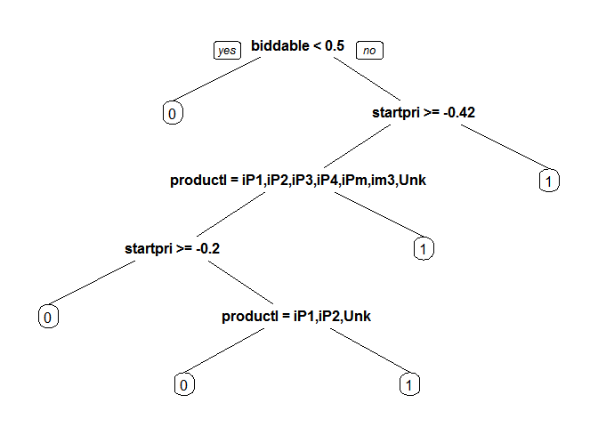
Now look at the results obtained using the CART model.
library(rpart) library(rpart.plot) model_cart1 <- rpart(sold ~ ., data = train, method = "class") prp(model_cart1) predict_cart <- predict(model_cart1, newdata = test, type = "prob")[,2] ROCRpred = prediction(predict_cart, test$sold) as.numeric(performance(ROCRpred, "auc")@y.values) ## [1] 0.8222028 The model makes the assessment worse than the previous one. Let's try to improve the results using the selection of parameters by cross-validation . We will select the parameter cp , which determines the complexity of the model
library(caret) ## Loading required package: lattice ## Loading required package: ggplot2 ## ## Attaching package: 'ggplot2' ## ## The following object is masked from 'package:NLP': ## ## annotate library(e1071) tr.control = trainControl(method = "cv", number = 10) cpGrid = expand.grid( .cp = seq(0.0001,0.01,0.001)) train(sold ~ ., data = train, method = "rpart", trControl = tr.control, tuneGrid = cpGrid ) ## CART ## ## 1303 samples ## 29 predictor ## 2 classes: '0', '1' ## ## No pre-processing ## Resampling: Cross-Validated (10 fold) ## ## Summary of sample sizes: 1173, 1172, 1172, 1173, 1173, 1173, ... ## ## Resampling results across tuning parameters: ## ## cp Accuracy Kappa Accuracy SD Kappa SD ## 0.0001 0.7674163 0.5293876 0.02132149 0.04497423 ## 0.0011 0.7743335 0.5430455 0.01594698 0.03388680 ## 0.0021 0.7896359 0.5714294 0.03938328 0.08143665 ## 0.0031 0.7957780 0.5831451 0.04394428 0.09055433 ## 0.0041 0.7919612 0.5748735 0.03867687 0.07958997 ## 0.0051 0.7934997 0.5775611 0.03727279 0.07705049 ## 0.0061 0.7888843 0.5678360 0.03868024 0.08040614 ## 0.0071 0.7881210 0.5662543 0.03710725 0.07714919 ## 0.0081 0.7888902 0.5678010 0.03657083 0.07592070 ## 0.0091 0.7888902 0.5678010 0.03657083 0.07592070 ## ## Accuracy was used to select the optimal model using the largest value. ## The final value used for the model was cp = 0.0031. Insert the proposed value and evaluate the resulting model.
bestcp <- train(sold ~ ., data = train, method = "rpart", trControl = tr.control, tuneGrid = cpGrid )$bestTune model_cart2 <- rpart(sold ~ ., data = train, method = "class", cp = bestcp) predict_cart <- predict(model_cart2, newdata = test, type = "prob")[,2] ROCRpred = prediction(predict_cart, test$sold) as.numeric(performance(ROCRpred, "auc")@y.values) ## [1] 0.8021447 Random forest
Let's look at the results of the most difficult model in theory, but very simple to use - Random Forest
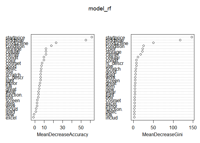
library(randomForest) ## randomForest 4.6-10 ## Type rfNews() to see new features/changes/bug fixes. ## ## Attaching package: 'randomForest' ## ## The following object is masked from 'package:dplyr': ## ## combine set.seed(1000) model_rf <- randomForest(sold ~ ., data = train, importance = T) predict_rf <- predict(model_rf, newdata = test, type = "prob")[,2] ROCRpred = prediction(predict_rf, test$sold) as.numeric(performance(ROCRpred, "auc")@y.values) ## [1] 0.8576486 As you can see, the model already shows the best results of all used. Let's try to improve it by eliminating unnecessary variables. The presence of a built-in assessment of the importance of variables in the model will help us.
varImpPlot(model_rf) On the left graph, we see that there is a feature that does not improve the quality of the model. Remove it and evaluate the resulting model.
set.seed(1000) model_rf2 <- randomForest(sold ~ .-excel, data = train, importance = T) predict_rf <- predict(model_rf2, newdata = test, type = "prob")[,2] ROCRpred = prediction(predict_rf, test$sold) as.numeric(performance(ROCRpred, "auc")@y.values) ## [1] 0.8566796 The assessment showed that there was no improvement in the model, but, based on common sense, I believe that having the word excel in the product description is unlikely to affect sales, and simplifying the model (without significant damage to quality) improves its interpretation.
Thus, the best results from all the models studied were logistic regression. As a result, on the Public Board (50% estimate of all available test data), the model with a score of 0.84724 ranked 211 out of 1884, but dropped to 1291 in the final protocol.
Next time I plan to talk about how the quality of the model is influenced by the size of the training sample using the example of the Digit Recognizer task, and the application of the principal component method in the same task. Then I will talk about the experience of participating in the Bag of Words Meets Bags of Popcorn competition, as well as a long study in the well-known task Titanic: Machine Learning from Disaster , in which I will tell you about how knowledge about Titanic and the catastrophe help solve the problem.
And finally, I recommend to sign up for the guys on the course on data analysis . In my experience:
- Only useful practical methods are given.
- The emphasis is on the result to be achieved in the tasks, and not just the solution
- Really motivates and makes a lot of work
See you!
Source: https://habr.com/ru/post/266421/
All Articles