Overview of segmentation algorithms
This summer I was lucky enough to get a summer internship at Itseez . I was asked to explore modern methods that would allow to select the locations of objects in the image. Basically, these methods rely on segmentation, so I began my work with an introduction to this area of computer vision.
Image segmentation is the division of an image into multiple areas covering it. Segmentation is used in many areas, for example, in manufacturing to indicate defects in the assembly of parts, in medicine for the initial processing of images, as well as for the mapping of the terrain from satellite images. For those who are interested in understanding how such algorithms work, welcome under cat. We will look at several methods from the OpenCV computer vision library .
Water Segmentation Segmentation Algorithm (WaterShed)
The algorithm works with an image as with a function of two variables f = I (x, y) , where x, y are the coordinates of a pixel:
')
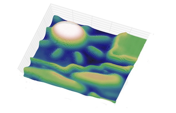
The value of the function can be the intensity or modulus of the gradient. For the greatest contrast, you can take a gradient from the image. If the absolute value of the gradient is plotted along the OZ axis, then ridges form at the places of intensity drop, and plains in homogeneous regions. After finding the minima of the function f , there is a process of filling with “water”, which begins with a global minimum. As soon as the water level reaches the value of the next local minimum, its filling with water begins. When the two regions begin to merge, a partition is built to prevent the regions from merging [2]. The water will continue to rise until the regions are separated only by artificially constructed partitions (Fig. 1).
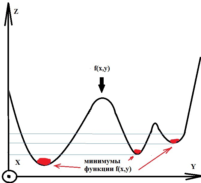
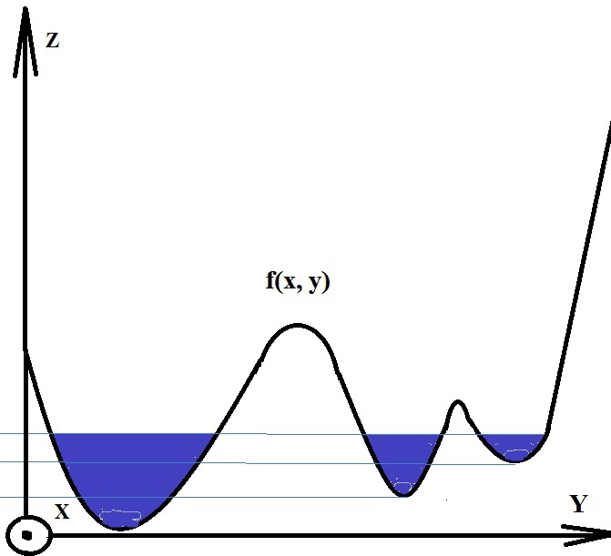
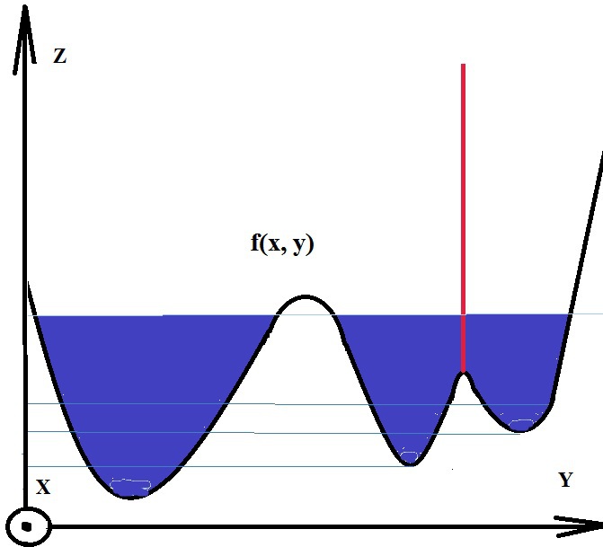
Fig.1. Illustration of the water filling process
Such an algorithm can be useful if there are a small number of local minima in the image, and in the case of a large number of them there is an excessive splitting into segments. For example, if you directly apply the algorithm to fig. 2, we obtain many small parts of fig. 3
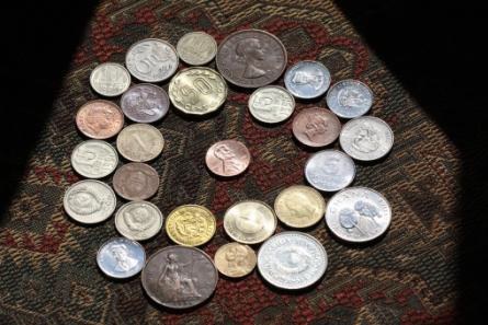
Fig. 2. Original image
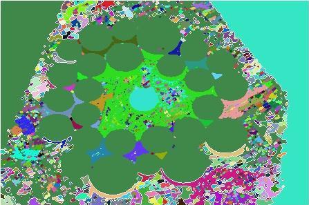
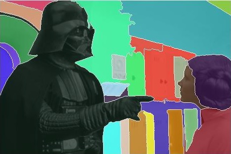
Fig. 3. Image after segmentation with WaterShed algorithm
How to cope with small details?
To get rid of the excess of small parts, you can specify areas that will be tied to the nearest minimum. The partition will be built only if the two regions merge with the markers, otherwise merging of these segments will occur. This approach removes the effect of redundant segmentation, but requires pre-processing of the image to highlight markers that can be labeled interactively in the image in Fig. 4, 5.
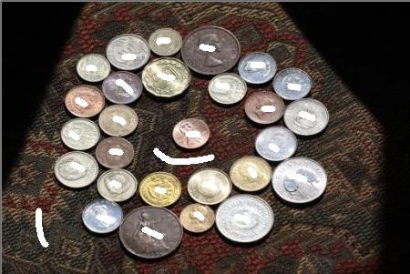
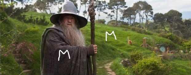
Fig. 4. Image with markers
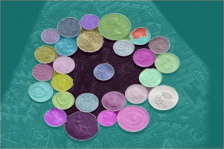
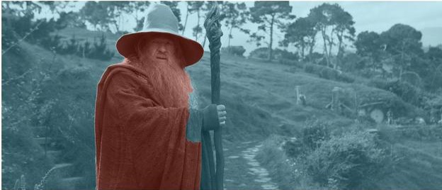
Fig. 5. Image after segmentation with WaterShed using markers
If it is required to act automatically without user intervention, then you can use, for example, the findContours () function to select markers, but here, too, for better segmentation, small contours should be deleted. 6., for example, removing them along the threshold along the contour length. Or, before separating outlines, use dilated erosion to remove small parts.
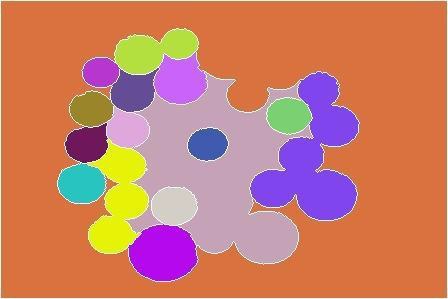
Fig. 6. As the markers were used contours having a length above a certain threshold.
Fig. 4. Image with markers
Fig. 5. Image after segmentation with WaterShed using markers
If it is required to act automatically without user intervention, then you can use, for example, the findContours () function to select markers, but here, too, for better segmentation, small contours should be deleted. 6., for example, removing them along the threshold along the contour length. Or, before separating outlines, use dilated erosion to remove small parts.
Fig. 6. As the markers were used contours having a length above a certain threshold.
As a result of the algorithm, we get a mask with a segmented image, where the pixels of one segment are marked with the same label and form a connected area. The main disadvantage of this algorithm is the use of a preprocessing procedure for images with a large number of local minima (images with a complex texture and with an abundance of different colors).
Sample code to run the algorithm:
Mat image = imread("coins.jpg", CV_LOAD_IMAGE_COLOR); // Mat imageGray, imageBin; cvtColor(image, imageGray, CV_BGR2GRAY); threshold(imageGray, imageBin, 100, 255, THRESH_BINARY); std::vector<std::vector<Point> > contours; std::vector<Vec4i> hierarchy; findContours(imageBin, contours, hierarchy, CV_RETR_TREE, CV_CHAIN_APPROX_SIMPLE); Mat markers(image.size(), CV_32SC1); markers = Scalar::all(0); int compCount = 0; for(int idx = 0; idx >= 0; idx = hierarchy[idx][0], compCount++) { drawContours(markers, contours, idx, Scalar::all(compCount+1), -1, 8, hierarchy, INT_MAX); } std::vector<Vec3b> colorTab(compCount); for(int i = 0; i < compCount; i++) { colorTab[i] = Vec3b(rand()&255, rand()&255, rand()&255); } watershed(image, markers); Mat wshed(markers.size(), CV_8UC3); for(int i = 0; i < markers.rows; i++) { for(int j = 0; j < markers.cols; j++) { int index = markers.at<int>(i, j); if(index == -1) wshed.at<Vec3b>(i, j) = Vec3b(0, 0, 0); else if (index == 0) wshed.at<Vec3b>(i, j) = Vec3b(255, 255, 255); else wshed.at<Vec3b>(i, j) = colorTab[index - 1]; } } imshow("watershed transform", wshed); waitKey(0); MeanShift Segmentation Algorithm
MeanShift groups objects with similar attributes. Pixels with similar features are combined into one segment, the output is an image with homogeneous areas.

For example, as coordinates in feature space, you can select pixel coordinates (x, y) and RGB pixel components. By depicting pixels in the feature space, you can notice thickening in certain places.
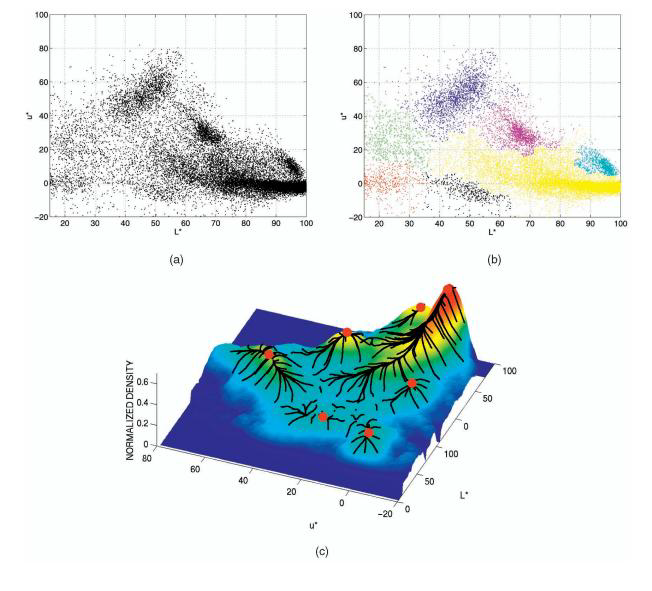
Fig. 7. (a) Pixels in a two-dimensional feature space. (b) Pixels that came to one local maximum are painted in one color. (with)
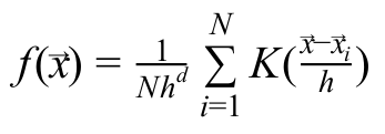
To make it easier to describe point condensations, a density function is introduced:
Gradient Estimation of Density Function
To estimate the density function gradient, one can use the mean shift vector 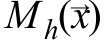
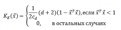
As a core OpenCV uses the Epechnikov kernel [4]:
 Is the volume of the d- dimensional sphere with a unit radius.
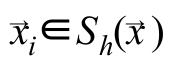 means that the sum goes not for all pixels, but only for those that fall into a sphere of radius h with the center at the point where the vector points
  in the space of signs [4]. This is introduced specifically to reduce the amount of computation.
  - the volume of the d- dimensional sphere with radius h. You can separately set the radius for the spatial coordinates and the radius separately in the color space.
  - the number of pixels that fall into the sphere. Magnitude
 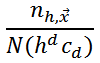 can be considered as an estimate of the value
  in the area of
  .
.
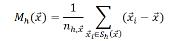
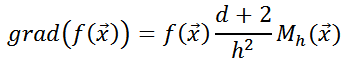
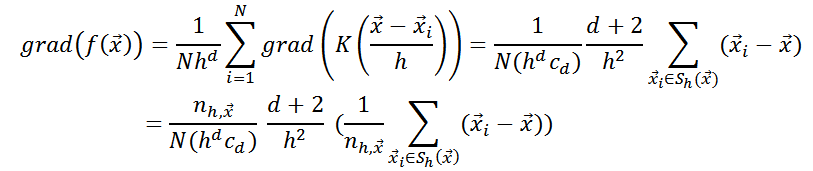
Therefore, in order to walk along the gradient, it suffices to calculate the value - vector of the average shift. It should be remembered that when choosing a different core, the mean shift vector will look different.
As a core
- the number of pixels that fall into the sphere. Magnitude can be considered as an estimate of the value Therefore, in order to walk along the gradient, it suffices to calculate the value
When you select pixels as indications of coordinates and intensities in colors in one segment, pixels with similar colors and located close to each other will be combined. Accordingly, if you select another feature vector, then the union of the pixels into segments will already go along it. For example, if you remove the coordinates from the attributes, the sky and the lake will be considered as one segment, since the pixels of these objects in the attribute space would fall into one local maximum.
If the object that we want to select consists of areas that differ greatly in color, then MeanShift will not be able to combine these regions into one, and our object will consist of several segments. But well to cope with a uniform object in color on a variegated background. More MeanShift is used in the implementation of the tracking algorithm for moving objects [5].
Sample code to run the algorithm:
Result:
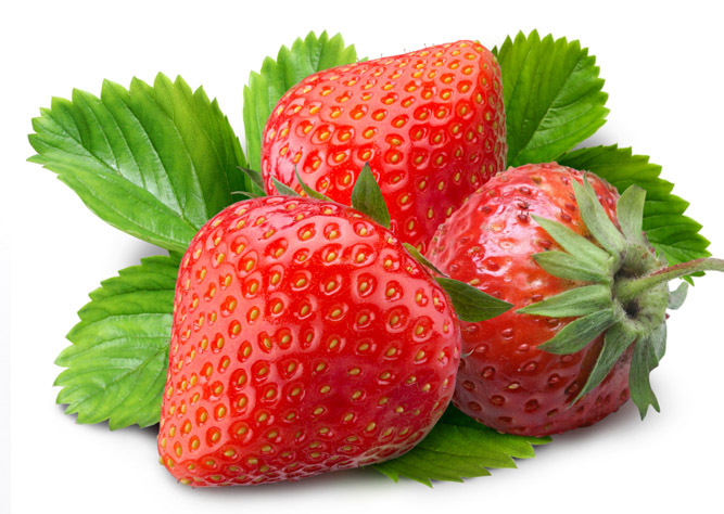
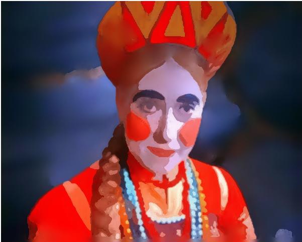
Fig. 8. Original image
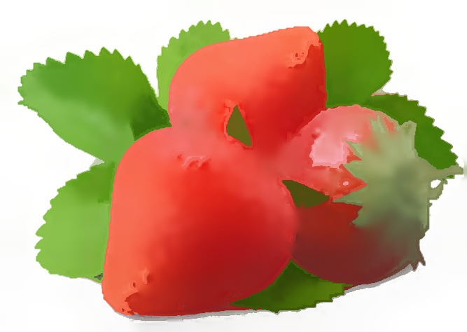
Fig. 9. After segmentation by MeanShift algorithm
Mat image = imread("strawberry.jpg", CV_LOAD_IMAGE_COLOR); Mat imageSegment; int spatialRadius = 35; int colorRadius = 60; int pyramidLevels = 3; pyrMeanShiftFiltering(image, imageSegment, spatialRadius, colorRadius, pyramidLevels); imshow("MeanShift", imageSegment); waitKey(0); Result:
Fig. 8. Original image
Fig. 9. After segmentation by MeanShift algorithm
FloodFill segmentation algorithm
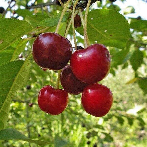
Using the FloodFill (fill or “flood” method) you can select regions of uniform color. To do this, select the starting pixel and set the interval for changing the color of neighboring pixels relative to the original. The interval can be asymmetric. The algorithm will combine the pixels into one segment (filling them with one color) if they fall within the specified range. The output will be a segment filled with a certain color, and its area in pixels.
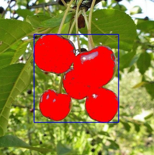
Such an algorithm can be useful for filling a region with weak color differences with a uniform background. One of the options for using FloodFill may be to identify the damaged edges of the object. For example, if the algorithm fills the neighboring regions, filling the homogeneous areas with a certain color, then the integrity of the boundary between these areas is violated. Below in the image you can see that the integrity of the borders of the filled areas is maintained:
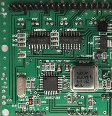
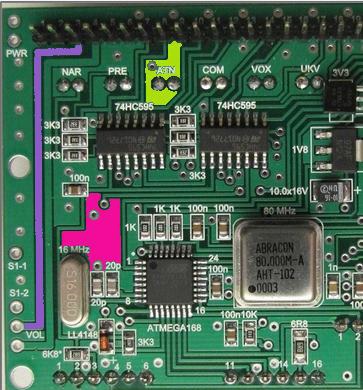
Fig. 10, 11. Original image and result after filling in several areas
And the following pictures show the version of the work of FloodFill in case of damage to one of the borders in the previous image.
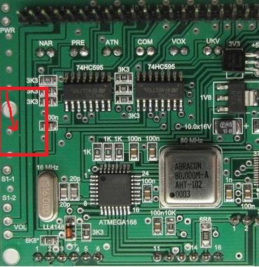
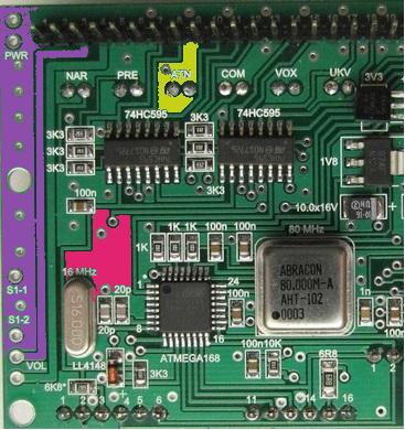
Fig. 12, 13. Illustration of the work of FloodFill in violation of the integrity of the boundary between the poured areas
Sample code to run the algorithm:
The number of filled pixels is written to the area variable.
Result:
Mat image = imread("cherry.jpg", CV_LOAD_IMAGE_COLOR); Point startPoint; startPoint.x = image.cols / 2; startPoint.y = image.rows / 2; Scalar loDiff(20, 20, 255); Scalar upDiff(5, 5, 255); Scalar fillColor(0, 0, 255); int neighbors = 8; Rect domain; int area = floodFill(image, startPoint, fillColor, &domain, loDiff, upDiff, neighbors); rectangle(image, domain, Scalar(255, 0, 0)); imshow("floodFill segmentation", image); waitKey(0); The number of filled pixels is written to the area variable.
Result:
GrabCut segmentation algorithm
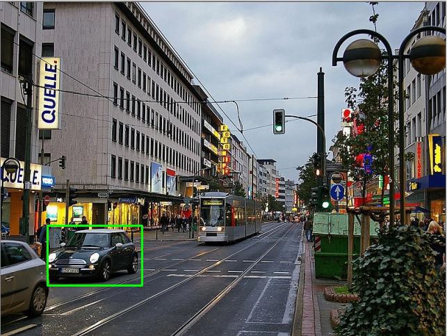
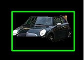
This is an interactive algorithm for selecting an object; it was developed as a more convenient alternative to the magnetic lasso (to select an object, the user needed to circle his path with the mouse). For the algorithm to work, it is enough to enclose the object together with a part of the background in a rectangle (grab). Segmentation of the object will occur automatically (cut).
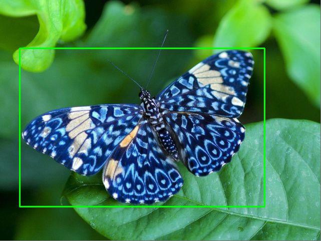
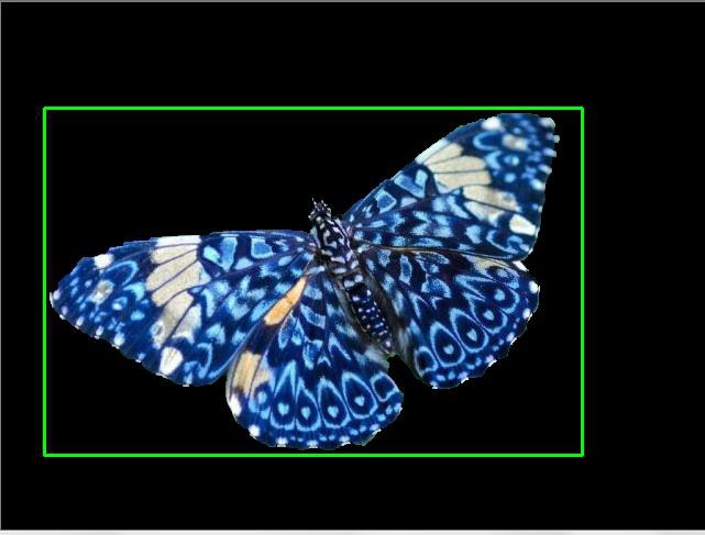
Difficulties may occur during segmentation if there are colors inside the bounding box that are found in large numbers not only in the object, but also in the background. In this case, you can put additional labels of the object (red line) and background (blue line).

Consider the idea of the algorithm. The basis is an algorithm of interactive segmentation GraphCut, where the user must put markers on the background and on the object. The image is treated as an array.
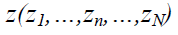 . Z - the intensity values of pixels, N is the total number of pixels. To separate an object from the background, the algorithm determines the values of the elements of the transparency array.
 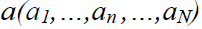 , and
, and  may take two values if = 0 , then the pixel belongs to the background, if = 1 , then the object. Internal parameter
  contains a histogram of the foreground intensity distribution and a histogram of the background:
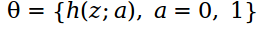 .
.Segmentation task - find unknowns
. The function of energy is considered:
Moreover, the minimum energy corresponds to the best segmentation.
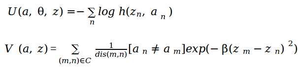
V (a, z) - the term is responsible for the connection between the pixels. The sum goes over all pairs of pixels that are neighbors, dis (m, n) is the Euclidean distance.
 responsible for the participation of pairs of pixels in the sum, if a n = a m , then this pair will not be taken into account.
Finding the global minimum of the energy function E , we get an array of transparency
 . To minimize the energy function, the image is described as a graph and a minimal cut of the graph is sought. Unlike GraphCut, in the GrabCut algorithm , pixels are considered in the RGB space, so the Gaussian Mixture Model (GMM) is used to describe color statistics. The work of the GrabCut algorithm can be viewed by running the OpenCV sample grabcut.cpp .
We considered only a small part of the existing algorithms. As a result of segmentation, areas are selected in the image into which pixels are combined according to selected features. FloodFill is suitable for filling objects of uniform color. With the task of separating a particular object from the background, GrabCut will do well . If you use the implementation of MeanShift from OpenCV, then pixels that are close in color and coordinates will be clustered. WaterShed is suitable for images with a simple texture. Thus, the segmentation algorithm should be chosen, of course, on the basis of a specific task.
Literature:
- G. Bradski, A. Kaehler Learning OpenCV: OReilly, second edition 2013
- R. Gonzalez, R. Woods Digital Image Processing, Moscow: Technosphere, 2005. - 1072 p.
- D. Comaniciu, P. Meer Mean Shift: A Robust Approach Toward Feature Space Analysis. IEEE Transactions on Pattern Analysis and Machine Intelligence, 2002, pp. 603–619.
- D. Comaniciu, P. Meer Mean shift analysis and applications, IEEE International Conference on Computer Vision, 1999, vol. 2, pp. 1197.
- D. Comaniciu, V. Ramesh, P. Meer Real-Time Tracking of Non-Rigid Objects Using Mean Shift, Conference on CVPR, 2000, vol. 2, pp. 1-8.
- S. Rother, V. Kolmogorov, A. Blake Grabcut - interactive foreground extraction using iterated graph cuts, 2004
- OpenCV samples
Source: https://habr.com/ru/post/266347/
All Articles