Visualization of static and dynamic networks on R, part 5
In the first part :
In the second part : colors and fonts in graphs R.
In the third part: the parameters of graphs, vertices and edges.
In the fourth part: network placement.
')
In this part: emphasis on network properties, vertices, edges, paths.
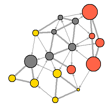
Please note that our network graph is still not very useful. We can determine the type and size of the vertices, but we can say little about the structure, since the edges are very closely spaced. One way to solve the problem is to see if the network can be “thinned out”, leaving only the most significant links and discarding the rest.
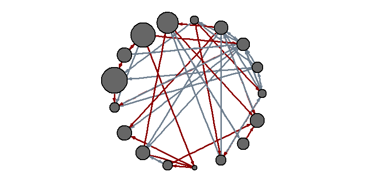
There are more complex ways to isolate key edges, but in this example we’ll leave only those that weigh more than the average for the network. In igraph, you can remove edges using
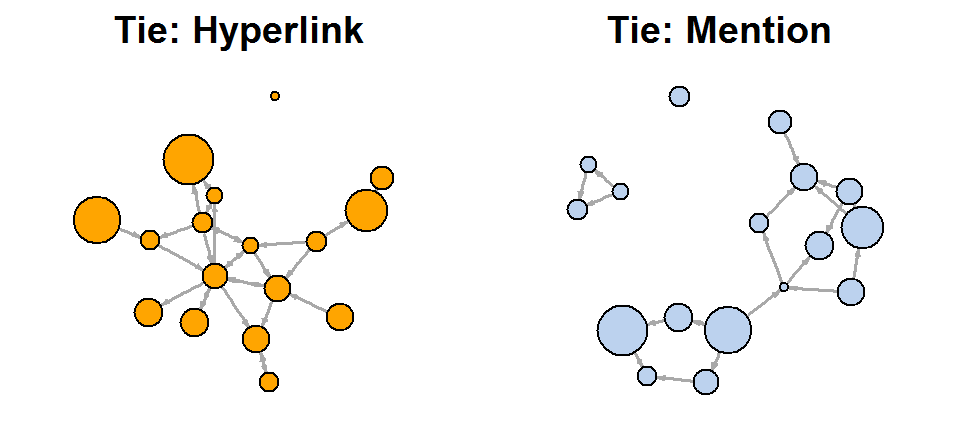
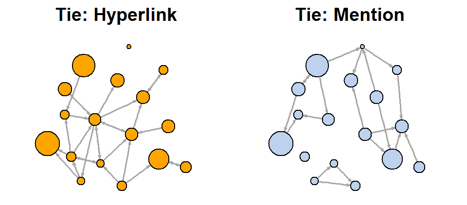
Another approach to solving a problem is to display two types of links (links and references) separately:
You can also try to make the network map more useful by showing the associations in it:
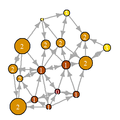
Sometimes you need to focus the visualization on a specific vertex or group of vertices. In our example of a media network, you can explore the distribution of information between central entities. For example, let's derive the distance from the NYT (New York Times). The
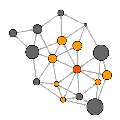
Or you can show all the closest neighbors WSJ (Wall Street Journal). Notice that the
Another way to draw attention to a group of vertices is to “tag” them:
You can also select the path on the network:
- network visualization: why? how?
- visualization parameters
- best practices - aesthetics and performance
- data formats and preparation
- description of the data sets used in the examples
- getting started with igraph
In the second part : colors and fonts in graphs R.
In the third part: the parameters of graphs, vertices and edges.
In the fourth part: network placement.
')
In this part: emphasis on network properties, vertices, edges, paths.
Emphasizing network properties
Please note that our network graph is still not very useful. We can determine the type and size of the vertices, but we can say little about the structure, since the edges are very closely spaced. One way to solve the problem is to see if the network can be “thinned out”, leaving only the most significant links and discarding the rest.
hist(links$weight) mean(links$weight) sd(links$weight) There are more complex ways to isolate key edges, but in this example we’ll leave only those that weigh more than the average for the network. In igraph, you can remove edges using
delete.edges(net, edges) : cut.off <- mean(links$weight) net.sp <- delete.edges(net, E(net)[weight<cut.off]) l <- layout.fruchterman.reingold(net.sp, repulserad=vcount(net)^2.1) plot(net.sp, layout=l) Another approach to solving a problem is to display two types of links (links and references) separately:
E(net)$width <- 1.5 plot(net, edge.color=c("dark red", "slategrey")[(E(net)$type=="hyperlink")+1], vertex.color="gray40", layout=layout.circle) net.m <- net - E(net)[E(net)$type=="hyperlink"] # net.h <- net - E(net)[E(net)$type=="mention"] par(mfrow=c(1,2)) plot(net.h, vertex.color="orange", main="Tie: Hyperlink") # : plot(net.m, vertex.color="lightsteelblue2", main="Tie: Mention") # : l <- layout.fruchterman.reingold(net) plot(net.h, vertex.color="orange", layout=l, main="Tie: Hyperlink") plot(net.m, vertex.color="lightsteelblue2", layout=l, main="Tie: Mention") dev.off() You can also try to make the network map more useful by showing the associations in it:
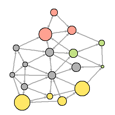
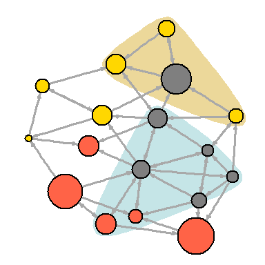
V(net)$community <- optimal.community(net)$membership colrs <- adjustcolor( c("gray50", "tomato", "gold", "yellowgreen"), alpha=.6) plot(net, vertex.color=colrs[V(net)$community]) Emphasizing some vertices or edges
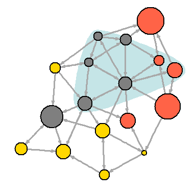
Sometimes you need to focus the visualization on a specific vertex or group of vertices. In our example of a media network, you can explore the distribution of information between central entities. For example, let's derive the distance from the NYT (New York Times). The
shortest.paths function (as the name shows) returns the matrix of shortest paths between vertices in the network. dist.from.NYT <- shortest.paths(net, algorithm="unweighted")[1,] oranges <- colorRampPalette(c("dark red", "gold")) col <- oranges(max(dist.from.NYT)+1)[dist.from.NYT+1] plot(net, vertex.color=col, vertex.label=dist.from.NYT, edge.arrow.size=.6, vertex.label.color="white") Or you can show all the closest neighbors WSJ (Wall Street Journal). Notice that the
neighbors function finds all vertices in one step from the center feature. A similar function that finds all the edges for a node is called incident . col <- rep("grey40", vcount(net)) col[V(net)$media=="Wall Street Journal"] <- "#ff5100" neigh.nodes <- neighbors(net, V(net)[media=="Wall Street Journal"], mode="out") col[neigh.nodes] <- "#ff9d00" plot(net, vertex.color=col) Another way to draw attention to a group of vertices is to “tag” them:
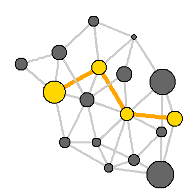
plot(net, mark.groups=c(1,4,5,8), mark.col="#C5E5E7", mark.border=NA) # : plot(net, mark.groups=list(c(1,4,5,8), c(15:17)), mark.col=c("#C5E5E7","#ECD89A"), mark.border=NA) You can also select the path on the network:
news.path <- get.shortest.paths(net, V(net)[media=="MSNBC"], V(net)[media=="New York Post"], mode="all", output="both") # : ecol <- rep("gray80", ecount(net)) ecol[unlist(news.path$epath)] <- "orange" # : ew <- rep(2, ecount(net)) ew[unlist(news.path$epath)] <- 4 # : vcol <- rep("gray40", vcount(net)) vcol[unlist(news.path$vpath)] <- "gold" plot(net, vertex.color=vcol, edge.color=ecol, edge.width=ew, edge.arrow.mode=0) Source: https://habr.com/ru/post/266285/
All Articles