Visualization of static and dynamic networks on R, part 4
In the first part :
In the second part : colors and fonts in graphs R.
In the third part: the parameters of graphs, vertices and edges.
In this part: network placement.
Network layouts are algorithms that return the coordinates of each vertex of the graph.
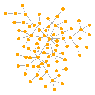
To study the locations, create a slightly larger graph, from 80 vertices. We use the barabasi.game function, which generates a simple graph starting from one vertex and increasing the vertices and edges depending on the specified level of preferred connection (how many more new objects will they prefer to communicate with the more popular nodes on the network).

')
You can set the location in the build function:

Or calculate the coordinates of the vertices in advance:


This placement is only an example, it is not very useful. Fortunately, there is a set of built-in placements in igraph, including:


Frühterman-Rheingold is one of the most commonly used power placement algorithms.
Power placement involves the creation of a beautiful graph with edges of the same length and the minimum possible number of intersections. They represent the graph as a physical system. Vertices are electrically charged particles that repel each other when they are too close. The ribs behave like springs, attracting connected vertices closer to each other. As a result, the vertices are evenly distributed over the chart area, and the placement is intuitive in the sense that the vertices with a large number of connections are closer to each other. The disadvantage of these algorithms is that they are rather slow, and therefore rarely used on graphs with more than 1000 vertices.
Here are some parameters that can be set for this placement:
You can also use the "weight" parameter, which increases the force of attraction between the vertices connected by heavier ribs.
You will notice that the placement is not strictly defined — different starts result in slightly different configurations. Preserving the placement of
Placing

Another popular power placement algorithm that shows good results for connected graphs is Kamada-Kawai. Like Frühterman-Rheingold, his goal is to minimize energy in the spring system. Igraph also contains a spring-based

The LGL (Large Graph Layout) Algorithm is designed for large connected graphs. It also allows you to set the root - the vertex, which will be located in the center of the placement.
By default, the coordinates of the graphs are scaled to the interval [-1,1] in both x and y. This can be changed using the

By default, igraph uses
Let's look at the layouts available in igraph:

- network visualization: why? how?
- visualization parameters
- best practices - aesthetics and performance
- data formats and preparation
- description of the data sets used in the examples
- getting started with igraph
In the second part : colors and fonts in graphs R.
In the third part: the parameters of graphs, vertices and edges.
In this part: network placement.
Network placement
Network layouts are algorithms that return the coordinates of each vertex of the graph.
To study the locations, create a slightly larger graph, from 80 vertices. We use the barabasi.game function, which generates a simple graph starting from one vertex and increasing the vertices and edges depending on the specified level of preferred connection (how many more new objects will they prefer to communicate with the more popular nodes on the network).
net.bg <- barabasi.game(80) V(net.bg)$frame.color <- "white" V(net.bg)$color <- "orange" V(net.bg)$label <- "" V(net.bg)$size <- 10 E(net.bg)$arrow.mode <- 0 plot(net.bg) ')
You can set the location in the build function:
plot(net.bg, layout=layout.random) Or calculate the coordinates of the vertices in advance:
l <- layout.circle(net.bg) plot(net.bg, layout=l) l is the x- and y-coordinate matrix (N x 2) for N vertices of the graph. You can easily set them yourself: l <- matrix(c(1:vcount(net.bg), c(1, vcount(net.bg):2)), vcount(net.bg), 2) plot(net.bg, layout=l) This placement is only an example, it is not very useful. Fortunately, there is a set of built-in placements in igraph, including:
# l <- layout.random(net.bg) plot(net.bg, layout=l) # l <- layout.circle(net.bg) plot(net.bg, layout=l) # 3D- l <- layout.sphere(net.bg) plot(net.bg, layout=l) Frühterman-Rheingold is one of the most commonly used power placement algorithms.
Power placement involves the creation of a beautiful graph with edges of the same length and the minimum possible number of intersections. They represent the graph as a physical system. Vertices are electrically charged particles that repel each other when they are too close. The ribs behave like springs, attracting connected vertices closer to each other. As a result, the vertices are evenly distributed over the chart area, and the placement is intuitive in the sense that the vertices with a large number of connections are closer to each other. The disadvantage of these algorithms is that they are rather slow, and therefore rarely used on graphs with more than 1000 vertices.
Here are some parameters that can be set for this placement:
area (by default - the square of the number of vertices) and repulserad (the radius of suppression for repulsion - area multiplied by the number of vertices). Both parameters affect the location of the chart - change them until you are satisfied with the result.You can also use the "weight" parameter, which increases the force of attraction between the vertices connected by heavier ribs.
You will notice that the placement is not strictly defined — different starts result in slightly different configurations. Preserving the placement of
l allows you to get the same result many times, which can be useful if you need to build a graph change in time or different relationships - and you need to leave the vertices on the same places in several graphs.Placing
fruchterman.reingold.grid similar to fruchterman.reingold , but faster. l <- layout.fruchterman.reingold(net.bg, repulserad=vcount(net.bg)^3, area=vcount(net.bg)^2.4) par(mfrow=c(1,2), mar=c(0,0,0,0)) # - 1 , 2 plot(net.bg, layout=layout.fruchterman.reingold) plot(net.bg, layout=l) dev.off() # , . Another popular power placement algorithm that shows good results for connected graphs is Kamada-Kawai. Like Frühterman-Rheingold, his goal is to minimize energy in the spring system. Igraph also contains a spring-based
layout.spring() called layout.spring() . l <- layout.kamada.kawai(net.bg) plot(net.bg, layout=l) l <- layout.spring(net.bg, mass=.5) plot(net.bg, layout=l) The LGL (Large Graph Layout) Algorithm is designed for large connected graphs. It also allows you to set the root - the vertex, which will be located in the center of the placement.
plot(net.bg, layout=layout.lgl) By default, the coordinates of the graphs are scaled to the interval [-1,1] in both x and y. This can be changed using the
rescale=FALSE parameter and manually scale the graph by multiplying the coordinates by a number. The layout.norm function allows layout.norm to normalize the graph to the desired boundaries. l <- layout.fruchterman.reingold(net.bg) l <- layout.norm(l, ymin=-1, ymax=1, xmin=-1, xmax=1) par(mfrow=c(2,2), mar=c(0,0,0,0)) plot(net.bg, rescale=F, layout=l*0.4) plot(net.bg, rescale=F, layout=l*0.6) plot(net.bg, rescale=F, layout=l*0.8) plot(net.bg, rescale=F, layout=l*1.0) dev.off() By default, igraph uses
layout.auto . It automatically selects the required placement algorithm based on the properties of the graph (size and connectivity).Let's look at the layouts available in igraph:
layouts <- grep("^layout\\.", ls("package:igraph"), value=TRUE) # , . layouts <- layouts[!grepl("bipartite|merge|norm|sugiyama", layouts)] par(mfrow=c(3,3)) for (layout in layouts) { print(layout) l <- do.call(layout, list(net)) plot(net, edge.arrow.mode=0, layout=l, main=layout) } dev.off() Source: https://habr.com/ru/post/266199/
All Articles