Generators of discretely distributed random variables
This article is a continuation of the post Generators of continuously distributed random variables . This chapter takes into account that all the theorems from the previous article have already been proved and the generators mentioned in it have already been implemented. As before, we have a certain basic generator of natural numbers from 0 to RAND_MAX:
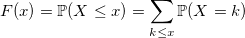
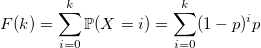
With discrete values, everything is more intuitive. The distribution function of a discrete random variable:
Despite the simplicity of the distribution of discrete random variables, it is sometimes more difficult to generate them, rather than continuous ones. We begin, as last time, with a trivial example.
')
Perhaps the fastest of the obvious ways to generate a random variable with a Bernoulli distribution is to do it in a similar way (all generators return double only for the unity of the interface):
Sometimes you can do it faster. “Sometimes” means “in the case in which the parameter p is a power 1/2”. The fact is that if the integer returned by the BasicRandGenerator () function is a uniformly distributed random variable, then every bit of it is equally distributed. This means that in the binary representation the number consists of bits distributed across Bernoulli. Since in these articles the base generator function returns unsigned long long, we have 64 bits. Here is a trick you can turn for p = 1/2:
If the operation time of the BasicRandGenerator () function is not sufficiently small, and cryptostability and the size of the generator period can be neglected, then for such cases there is an algorithm using only one uniformly distributed random variable for any sample size from the Bernoulli distribution:
I am sure that any of you will remember that his first random integer generator from a to b looked like this:
Well, and this is quite the right decision. With the only and not always correct assumption - you have a good basic generator. If it is defective like the old C-shny rand (), then you will get an even number for an odd number each time. If you do not trust your generator, then write this way:
It should also be noted that the distribution will not be completely even if RAND_MAX is not divided by the length of the interval b - a + 1 completely. However, the difference will not be so significant if this length is small enough.


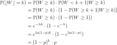
A random variable with a geometric distribution with the parameter p is a random variable with an exponential distribution with the parameter -ln (1 - p), rounded down to the nearest integer.
Can it be done faster? Sometimes. Let's look at the distribution function:
and use the ordinary inversion method: generate a standard uniformly distributed random variable U and return the minimum value of k for which this sum is greater than U:
Such a consistent search is quite effective, given that the values of a random variable with a geometric distribution are concentrated near zero. The algorithm, however, quickly loses its speed with too small values of p, and in this case it is better to use the exponential generator.
There is a secret. The values of p, (1-p) * p, (1-p) ^ 2 * p, ... can be calculated in advance and memorized. The question is where to stay. And then the geometric distribution property, which it inherited from the exponential - the lack of memory:

Thanks to this property, you can remember only a few first values (1-p) ^ i * p and then use recursion:

By definition, a random variable with a binomial distribution is the sum of n random variables with a Bernoulli distribution:
However, there is a linear dependence on n that needs to be circumvented. You can use the theorem: if Y_1, Y_2, ... are random variables with a geometric distribution with the parameter p and X is the smallest integer, such that:
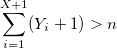
then X has a binomial distribution.
The running time of the next code grows only with increasing n * p.
And yet, the time complexity is growing.
The binomial distribution has one feature. As n grows, it tends to a normal distribution, or, if p ~ 1 / n, it tends to a Poisson distribution. Having generators for these distributions, they can replace the generator for the binomial in such cases. But what if this is not enough? In the Luc Devroye book "Non-Uniform Random Variate Generation" there is an example of an algorithm that works equally fast for any large n * p values. The idea of the algorithm is to sample with a deviation using normal and exponential distributions. Unfortunately, the story about the operation of this algorithm will be too large for this article, but in this book it is fully described.
If W_i is a random variable with standard exponential distribution with density lambda, then:
Using this property, you can write a generator in terms of a sum of exponentially distributed values with a density rate:
The Knut algorithm is based on this property. Instead of the sum of exponential values, each of which can be obtained by the inversion method using -ln (U), the product of uniform random variables is used:

and then:

Remembering in advance the value of exp (-rate), sequentially multiply U_i until the product exceeds it.
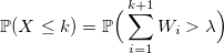
You can use the generation of only one random variable and the method of inversion:

It is better to start the search for k satisfying this condition with the most probable value, that is, with a floor (rate). We compare U with the probability that X <floor (rate) and go up if U is more, or down in another case:
The problem of all three generators in one - their complexity grows with the density parameter. But there is a salvation - for large values of density, the Poisson distribution tends to a normal distribution. You can also use a complex algorithm from the above-mentioned book “Non-Uniform Random Variate Generation”, well, or simply approximate, neglecting accuracy in the name of speed (depending on what the task is).
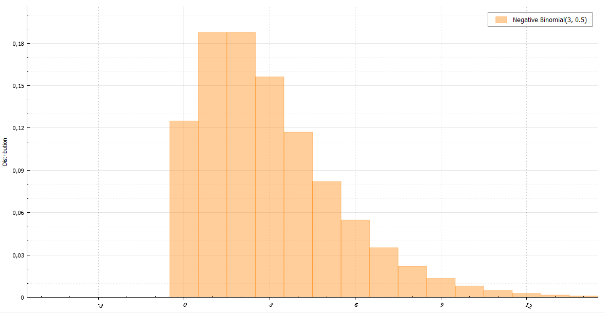
The negative binomial distribution is also referred to as the Pascal distribution (if r is integer) and the Field distribution (if r can be real). Using the characteristic function, it is easy to prove that the Pascal distribution is the sum of r geometrically distributed quantities with the parameter 1 - p:
The problem with this algorithm is obvious - linear dependence on r. We need something that will work equally well with any parameter. And this will help us a great property. If the random variable X has a Poisson distribution:

where density is random and has a gamma distribution:
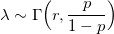
then X has a negative binomial distribution. Therefore, it is sometimes called the Poisson gamma distribution.
Now, we can quickly write a random value generator with Pascal distribution for large values of the parameter r.
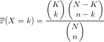
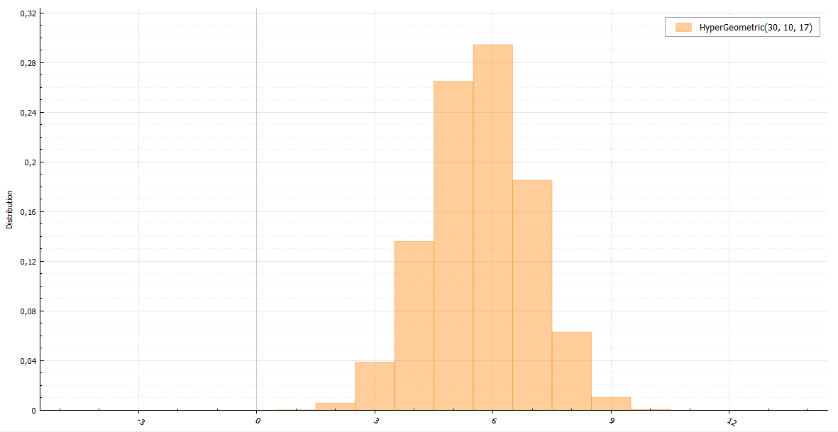
Imagine that there are N balls in the urn and K of them are white. You pull n balls. The number of whites among them will have a hypergeometric distribution. In general, it is better to take an algorithm using this definition:
Or you can use a sample with a deviation through the binomial distribution with parameters:
and constant M:
The algorithm with the binomial distribution works well in extreme cases for large n and even larger N (such that n << N). Otherwise, it is better to use the previous one, despite its growing complexity with increasing input parameters.

There is a useful theorem for this distribution. If U and V are uniformly distributed random variables from 0 to 1, then
will have a logarithmic distribution.
To speed up the algorithm, you can use two tricks. First, if V> p, then X = 1, since p> = 1- (1-p) ^ U. Second: let q = 1- (1-p) ^ U, then if V> q, then X = 1, if V> q ^ 2, then X = 2, etc. Thus, it is possible to return the most probable values 1 and 2 without frequent counts of logarithms.
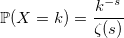
The denominator is the Riemann zeta function:

For zeta distribution, there is an algorithm that allows not to calculate the Riemannian zeta function. It is only necessary to be able to generate a Pareto distribution. Proof can be attached at the request of readers.
Finally, small algorithms for other complex distributions:
Implementing these and other C ++ generators 17
unsigned long long BasicRandGenerator() { unsigned long long randomVariable; // some magic here ... return randomVariable; } With discrete values, everything is more intuitive. The distribution function of a discrete random variable:
Despite the simplicity of the distribution of discrete random variables, it is sometimes more difficult to generate them, rather than continuous ones. We begin, as last time, with a trivial example.
')
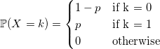
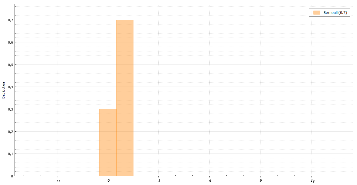
Bernoulli distribution
Perhaps the fastest of the obvious ways to generate a random variable with a Bernoulli distribution is to do it in a similar way (all generators return double only for the unity of the interface):
void setup(double p) { unsigned long long boundary = (1 - p) * RAND_MAX; // we storage this value for large sampling } double Bernoulli(double) { return BasicRandGenerator() > boundary; } Sometimes you can do it faster. “Sometimes” means “in the case in which the parameter p is a power 1/2”. The fact is that if the integer returned by the BasicRandGenerator () function is a uniformly distributed random variable, then every bit of it is equally distributed. This means that in the binary representation the number consists of bits distributed across Bernoulli. Since in these articles the base generator function returns unsigned long long, we have 64 bits. Here is a trick you can turn for p = 1/2:
double Bernoulli(double) { static const char maxDecimals = 64; static char decimals = 1; static unsigned long long X = 0; if (decimals == 1) { /// refresh decimals = maxDecimals; X = BasicRandGenerator(); } else { --decimals; X >>= 1; } return X & 1; } If the operation time of the BasicRandGenerator () function is not sufficiently small, and cryptostability and the size of the generator period can be neglected, then for such cases there is an algorithm using only one uniformly distributed random variable for any sample size from the Bernoulli distribution:
void setup(double p) { q = 1.0 - p; U = Uniform(0, 1); } double Bernoulli(double p) { if (U > q) { U -= q; U /= p; return 1.0; } U /= q; return 0.0; } Why does this algorithm work?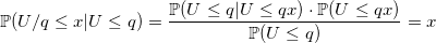

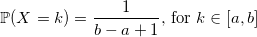
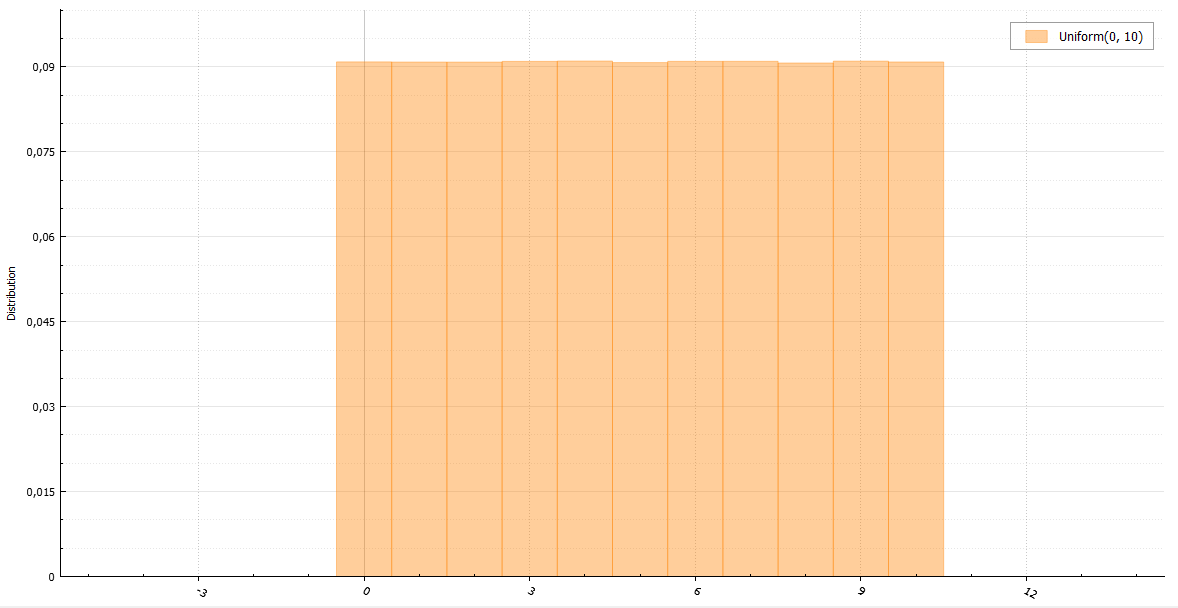
Uniform distribution
I am sure that any of you will remember that his first random integer generator from a to b looked like this:
double UniformDiscrete(int a, int b) { return a + rand() % (b - a + 1); } Well, and this is quite the right decision. With the only and not always correct assumption - you have a good basic generator. If it is defective like the old C-shny rand (), then you will get an even number for an odd number each time. If you do not trust your generator, then write this way:
double UniformDiscrete(int a, int b) { return a + round(BasicRandGenerator() * (b - a) / RAND_MAX); } It should also be noted that the distribution will not be completely even if RAND_MAX is not divided by the length of the interval b - a + 1 completely. However, the difference will not be so significant if this length is small enough.
Geometric distribution
A random variable with a geometric distribution with the parameter p is a random variable with an exponential distribution with the parameter -ln (1 - p), rounded down to the nearest integer.
Evidence
Let W be a random variable distributed exponentially with the -ln (1 - p) parameter. Then:
void setupRate(double p) { rate = -ln(1 - p); } double Geometric(double) { return floor(Exponential(rate)); } Can it be done faster? Sometimes. Let's look at the distribution function:
and use the ordinary inversion method: generate a standard uniformly distributed random variable U and return the minimum value of k for which this sum is greater than U:
double GeometricExponential(double p) { int k = 0; double sum = p, prod = p, q = 1 - p; double U = Uniform(0, 1); while (U < sum) { prod *= q; sum += prod; ++k; } return k; } Such a consistent search is quite effective, given that the values of a random variable with a geometric distribution are concentrated near zero. The algorithm, however, quickly loses its speed with too small values of p, and in this case it is better to use the exponential generator.
There is a secret. The values of p, (1-p) * p, (1-p) ^ 2 * p, ... can be calculated in advance and memorized. The question is where to stay. And then the geometric distribution property, which it inherited from the exponential - the lack of memory:
Thanks to this property, you can remember only a few first values (1-p) ^ i * p and then use recursion:
// works nice for p > 0.2 and tableSize = 16 void setupTable(double p) { table[0] = p; double prod = p, q = 1 - p; for (int i = 1; i < tableSize; ++i) { prod *= q; table[i] = table[i - 1] + prod; } } double GeometricTable(double p) { double U = Uniform(0, 1); /// handle tail by recursion if (U > table[tableSize - 1]) return tableSize + GeometricTable(p); /// handle the main body int x = 0; while (U > table[x]) ++x; return x; } Binomial distribution
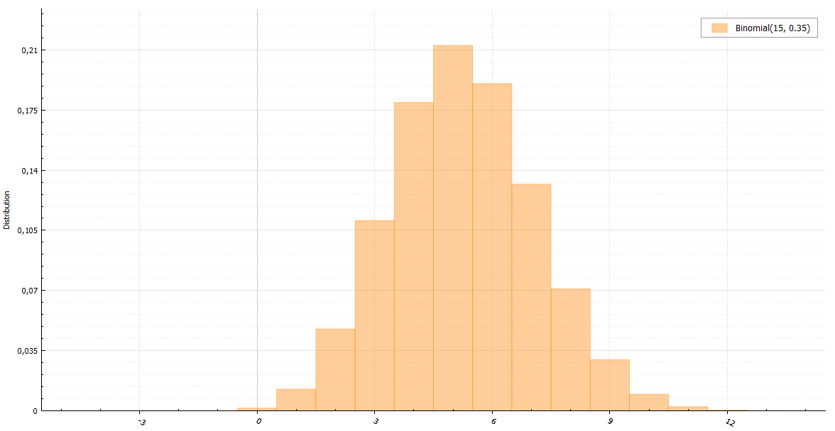
By definition, a random variable with a binomial distribution is the sum of n random variables with a Bernoulli distribution:
double BinomialBernoulli(double p, int n) { double sum = 0; for (int i = 0; i != n; ++i) sum += Bernoulli(p); return sum; } However, there is a linear dependence on n that needs to be circumvented. You can use the theorem: if Y_1, Y_2, ... are random variables with a geometric distribution with the parameter p and X is the smallest integer, such that:
then X has a binomial distribution.
Evidence
By definition, a random variable with a geometric distribution of Y is the number of Bernoulli's experiments before the first success. There is an alternative definition: Z = Y + 1 is the number of Bernoulli’s experiments up to and including the first success. This means that the sum of independent Z_i is the number of Bernoulli's experiments up to X + 1 success inclusive. And this sum is greater than n if and only if among the first n tests no more than X are successful. Respectively:

qed
qed
The running time of the next code grows only with increasing n * p.
double BinomialGeometric(double p, int n) { double X = -1, sum = 0; do { sum += Geometric(p) + 1.0; ++X; } while (sum <= n); return X; } And yet, the time complexity is growing.
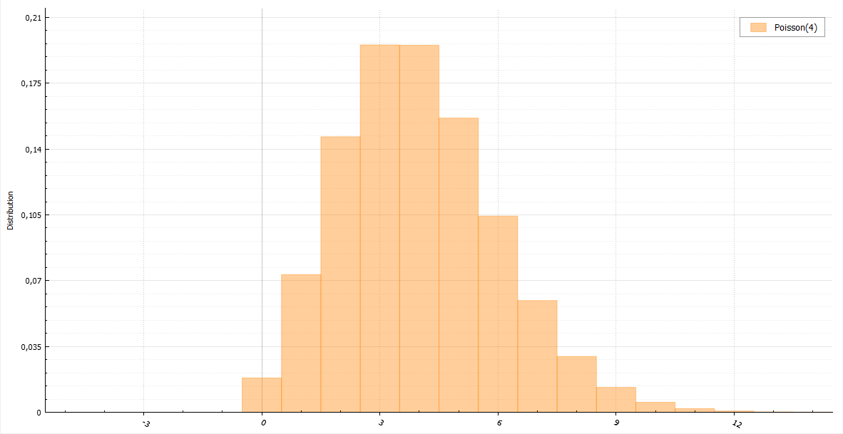
The binomial distribution has one feature. As n grows, it tends to a normal distribution, or, if p ~ 1 / n, it tends to a Poisson distribution. Having generators for these distributions, they can replace the generator for the binomial in such cases. But what if this is not enough? In the Luc Devroye book "Non-Uniform Random Variate Generation" there is an example of an algorithm that works equally fast for any large n * p values. The idea of the algorithm is to sample with a deviation using normal and exponential distributions. Unfortunately, the story about the operation of this algorithm will be too large for this article, but in this book it is fully described.
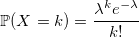
Poisson distribution
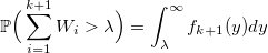
If W_i is a random variable with standard exponential distribution with density lambda, then:
Evidence
Let f_k (y) be the density of the standard Erlang distribution (sums of k standard exponentially distributed random variables):
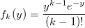
then
and the probability to get k:
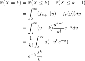
coincides with the Poisson distribution. qed
then
and the probability to get k:
coincides with the Poisson distribution. qed
Using this property, you can write a generator in terms of a sum of exponentially distributed values with a density rate:
double PoissonExponential(double rate) { int k = -1; double s = 0; do { s += Exponential(1); ++k; } while (s < rate); return k; } The Knut algorithm is based on this property. Instead of the sum of exponential values, each of which can be obtained by the inversion method using -ln (U), the product of uniform random variables is used:
and then:
Remembering in advance the value of exp (-rate), sequentially multiply U_i until the product exceeds it.
void setup(double rate) expRateInv = exp(-rate); } double PoissonKnuth(double) { double k = 0, prod = Uniform(0, 1); while (prod > expRateInv) { prod *= Uniform(0, 1); ++k; } return k; } You can use the generation of only one random variable and the method of inversion:
It is better to start the search for k satisfying this condition with the most probable value, that is, with a floor (rate). We compare U with the probability that X <floor (rate) and go up if U is more, or down in another case:
void setup(double rate) floorLambda = floor(rate); FFloorLambda = F(floorLamda); // P(X < floorLambda) PFloorLambda = P(floorLambda); // P(X = floorLambda) } double PoissonInversion(double) { double U = Uniform(0,1); int k = floorLambda; double s = FFloorLambda, p = PFloorLambda; if (s < U) { do { ++k; p *= lambda / k; s += p; } while (s < U); } else { s -= p; while (s > U) { p /= lambda / k; --k; s -= p; } } return k; } The problem of all three generators in one - their complexity grows with the density parameter. But there is a salvation - for large values of density, the Poisson distribution tends to a normal distribution. You can also use a complex algorithm from the above-mentioned book “Non-Uniform Random Variate Generation”, well, or simply approximate, neglecting accuracy in the name of speed (depending on what the task is).
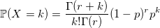
Negative binomial distribution
The negative binomial distribution is also referred to as the Pascal distribution (if r is integer) and the Field distribution (if r can be real). Using the characteristic function, it is easy to prove that the Pascal distribution is the sum of r geometrically distributed quantities with the parameter 1 - p:
double Pascal(double p, int r) { double x = 0; for (int i = 0; i != r; ++i) x += Geometric(1 - p); return x; } The problem with this algorithm is obvious - linear dependence on r. We need something that will work equally well with any parameter. And this will help us a great property. If the random variable X has a Poisson distribution:
where density is random and has a gamma distribution:
then X has a negative binomial distribution. Therefore, it is sometimes called the Poisson gamma distribution.
Evidence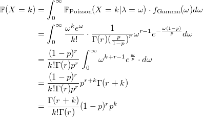
Now, we can quickly write a random value generator with Pascal distribution for large values of the parameter r.
double Pascal(double p, int r) { return Poisson(Gamma(r, p / (1 - p))); } Hypergeometric distribution
Imagine that there are N balls in the urn and K of them are white. You pull n balls. The number of whites among them will have a hypergeometric distribution. In general, it is better to take an algorithm using this definition:
double HyperGeometric(int N, int n, int K) { double sum = 0, p = static_cast<double>(K) / N; for (int i = 1; i <= n; ++i) { if (Bernoulli(p) && ++sum == K) return sum; p = (K - sum) / (N - i); } return sum; } Or you can use a sample with a deviation through the binomial distribution with parameters:
and constant M:
The algorithm with the binomial distribution works well in extreme cases for large n and even larger N (such that n << N). Otherwise, it is better to use the previous one, despite its growing complexity with increasing input parameters.
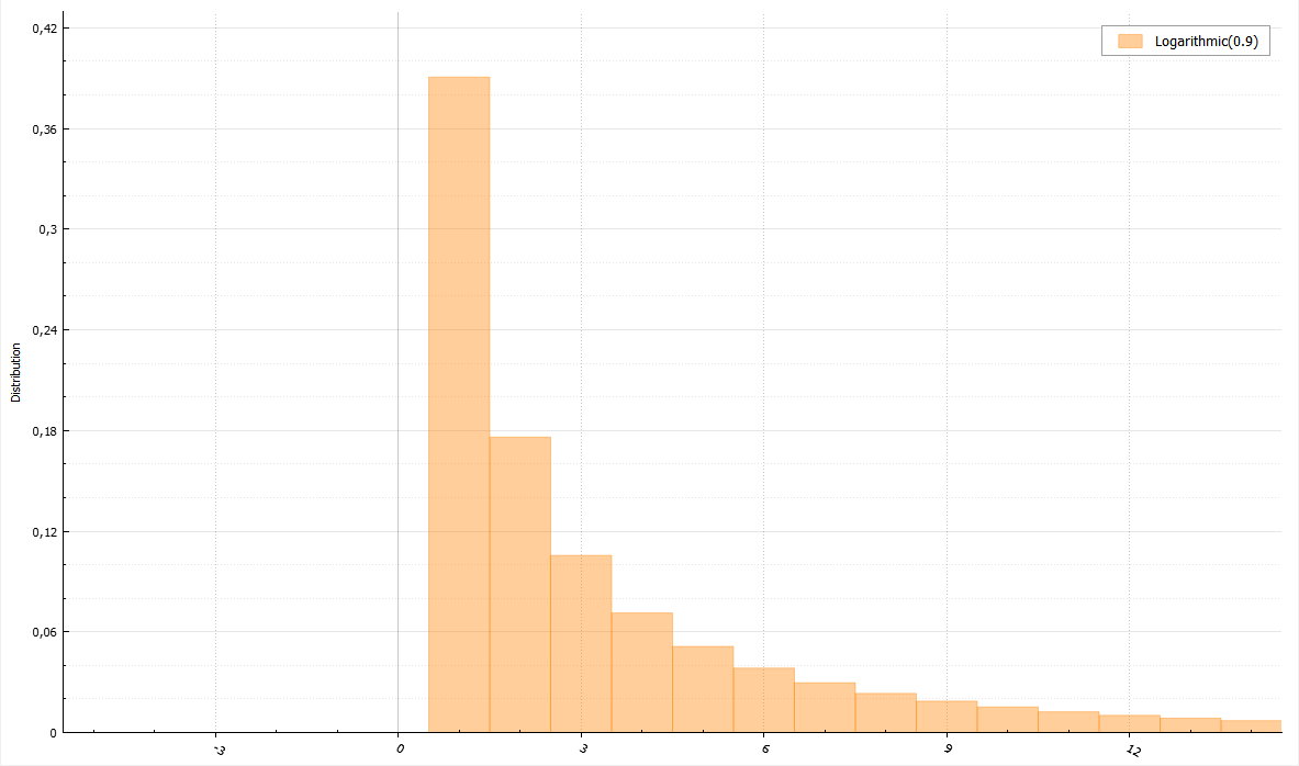
Logarithmic distribution
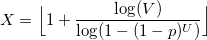
There is a useful theorem for this distribution. If U and V are uniformly distributed random variables from 0 to 1, then
will have a logarithmic distribution.
Evidence
Remembering the generators for the exponential and geometric distributions, it is easy to see that X, given by the formula above, satisfies the following distribution:

Let us prove that X has a logarithmic distribution:
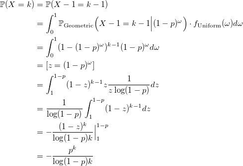
qed
Let us prove that X has a logarithmic distribution:
qed
To speed up the algorithm, you can use two tricks. First, if V> p, then X = 1, since p> = 1- (1-p) ^ U. Second: let q = 1- (1-p) ^ U, then if V> q, then X = 1, if V> q ^ 2, then X = 2, etc. Thus, it is possible to return the most probable values 1 and 2 without frequent counts of logarithms.
void setup(double p) { logQInv = 1.0 / log(1.0 - p); } double Logarithmic(double p) { double V = Uniform(0, 1); if (V >= p) return 1.0; double U = Uniform(0, 1); double y = 1.0 - exp(U / logQInv); if (V > y) return 1.0; if (V <= y * y) return floor(1.0 + log(V) / log(y)); return 2.0; } Zeta distribution
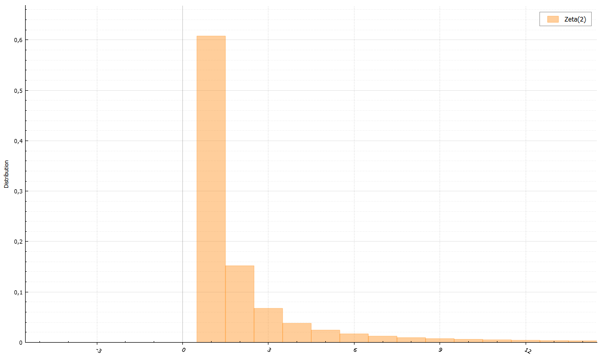
The denominator is the Riemann zeta function:
For zeta distribution, there is an algorithm that allows not to calculate the Riemannian zeta function. It is only necessary to be able to generate a Pareto distribution. Proof can be attached at the request of readers.
void setup(double s) { double sm1 = s - 1.0; b = 1 - pow(2.0, -sm1); } double Zeta(double) { /// rejection sampling from rounded down Pareto distribution int iter = 0; do { double X = floor(Pareto(sm1, 1.0)); double T = pow(1.0 + 1.0 / X, sm1); double V = Uniform(0, 1); if (V * X * (T - 1) <= T * b) return X; } while (++iter < 1e9); return NAN; /// doesn't work } Finally, small algorithms for other complex distributions:
double Skellam(double m1, double m2) { return Poisson(m1) - Poisson(m2); } double Planck(double a, double b) { double G = Gamma(a + 1, 1); double Z = Zeta(a + 1) return G / (b * Z); } double Yule(double ro) { double prob = 1.0 / Pareto(ro, 1.0); return Geometric(prob) + 1; } Implementing these and other C ++ generators 17
Source: https://habr.com/ru/post/265321/
All Articles