Determining the relationship between signs: Chi-square test

In this article, we will talk about the study of the relationship between signs, or whatever you like - random variables, variables. In particular, we will analyze how to introduce a measure of dependence between features using the Chi-square test and compare it with the correlation coefficient.

What can it be needed for? For example, in order to understand which signs are more dependent on the target variable when building credit scoring - determining the probability of a client’s default. Or, as in my case, understand what indicators need to be used for programming a trading robot.

Separately, I note that I use the c # language for data analysis. Perhaps this is all already implemented in R or Python, but using c # for me allows you to sort out the topic in detail, moreover it is my favorite programming language.

Let's start with a very simple example; let's create four columns in Excel using a random number generator:
X = CASE (-100; 100)
Y = X * 10 + 20
Z = X * X
T = CASE (-100; 100)
')


As you can see, the variable Y is linearly dependent on X ; variable Z is quadratically dependent on X ; the variables X and T are independent. I made this choice on purpose, because we will compare our measure of dependence with the correlation coefficient . As is known, between two random variables it is equal modulo 1 if between them the “hard” type of dependence is linear. There is no correlation between two independent random variables, but zero equality does not follow from the equality of the correlation coefficient . Further we will see it on the example of variables X and Z.

Save the file as data.csv and start the first look. To begin with, we calculate the correlation coefficient between the quantities. I did not embed the code in the article, it is on my github . We obtain a correlation for all possible pairs:



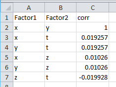
It can be seen that the linearly dependent X and Y correlation coefficient is equal to 1. But for X and Z it is equal to 0.01, although we have defined the explicit relationship Z = X * X. It is clear that we need a measure that “feels” the relationship better. But before proceeding to the Chi-square test, let's look at what a contingency matrix is.

To build a conjugation matrix, we divide the range of variable values ​​into intervals (or categorize). There are many ways to do this, and there is no universal one. Some of them are divided into intervals so that they fall into the same number of variables, others are divided into intervals of equal length. I personally have the spirit to combine these approaches. I decided to use this method: I deduct an estimate from the variable. expectations, then the resulting divide by the standard deviation estimate. In other words, I center and normalize the random variable. The resulting value is multiplied by a factor (in this example, it is equal to 1), after which everything is rounded to the whole. The output is a variable of type int, which is the class identifier.

So, take our signs of X and Z , categorize as described above, and then count the number and probability of occurrence of each class and the likelihood of the appearance of pairs of signs:



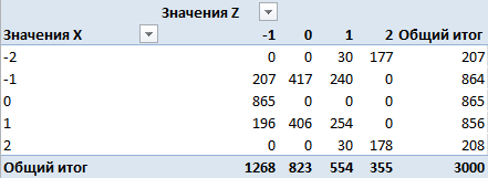
This is a matrix by quantity. Here in the rows - the number of occurrences of classes of the variable X , in the columns - the number of occurrences of classes of the variable Z , in the cells - the number of occurrences of pairs of classes at the same time. For example, class 0 met 865 times for variable X , 823 times for variable Z and never had a pair (0,0). We turn to the probabilities, dividing all values ​​by 3000 (the total number of observations):



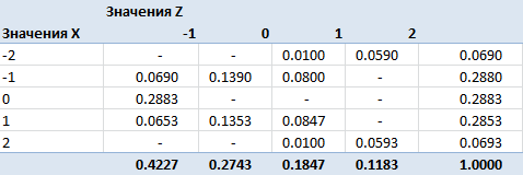
We obtained a contingency matrix obtained after categorizing the traits. Now it's time to think about the criterion. By definition, random variables are independent if the sigma-algebras generated by these random variables are independent. Independence of sigma-algebras implies pairwise independence of events from them. Two events are called independent if the probability of their joint occurrence is equal to the product of the probabilities of these events: Pij = Pi * Pj . It is this formula that we will use to construct the criterion.

Null hypothesis : categorized signs X and Z are independent. Equivalent to it: the distribution of the conjugacy matrix is ​​given exclusively by the probabilities of the occurrence of classes of variables (the probabilities of rows and columns). Or so: the cells of the matrix are the product of the corresponding probabilities of the rows and columns. We will use this formulation of the null hypothesis to construct a decision rule: a significant discrepancy between Pij and Pi * Pj will be the basis for rejecting the null hypothesis.

Let be - probability of occurrence of class 0 in variable X. In total, we have n classes for X and m classes for Z. It turns out that in order to specify the distribution of the matrix, we need to know these n and m probabilities. But in fact, if we know the n-1 probability for X , then the latter is found by subtracting from 1 the sum of the others. Thus, to find the distribution of the conjugacy matrix, we need to know the l = (n-1) + (m-1) values. Or we have an l- dimensional parametric space, the vector from which gives us our desired distribution. The chi-square statistic will look like this:

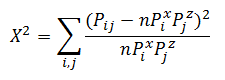
and, according to Fisher's theorem, have a Chi-square distribution with n * ml-1 = (n-1) (m-1) degrees of freedom.

Let us set a significance level of 0.95 (or the probability of an error of the first kind is 0.05). Find the quantile of the distribution of Chi for a given level of significance and degrees of freedom from the example (n-1) (m-1) = 4 * 3 = 12 : 21.02606982. The chi-square statistic itself for the variables X and Z is 4088.006631. It is seen that the hypothesis of independence is not accepted. It is convenient to consider the ratio of Chi-square statistics to the threshold value - in this case, it is equal to Chi2Coeff = 194.4256186 . If this ratio is less than 1, then the independence hypothesis is accepted; if more, then no. Find this relationship for all pairs of attributes:



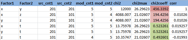
Here Factor1 and Factor2 are the names of the signs.
src_cnt1 and src_cnt2 - the number of unique values ​​of the original signs
mod_cnt1 and mod_cnt2 - the number of unique values ​​of attributes after categorization
chi2 - Chi-square statistics
chi2max is the chi-square statistic threshold for a significance level of 0.95
chi2Coeff - the ratio of the Chi-square statistic to the threshold value
corr - correlation coefficient

It can be seen that the following pairs of features, ( X, T ), ( Y, T ) and ( Z, T ), are independent (chi2coeff <1), which is logical, since the variable T is generated randomly. The variables X and Z are dependent, but less than linearly dependent X and Y , which is also logical.

I put the code for the utility that calculates these indicators on github, in the same place, the data.csv file. The utility takes a csv-file as input and calculates dependencies between all pairs of columns: PtProject.Dependency.exe data.csv

References:
1. Independence Hypothesis Testing: Pearson Chi-Square Test
2. Pearson Chi-square test for testing the parametric hypothesis
3. Implementation of the criterion on c #