Clustering graphs and searching for communities. Part 2: k-medoids and modifications

Hi, Habr! In this part we will describe to you the algorithm by which the colors on the graphs from the first part were obtained. The algorithm is based on k-medoids - a fairly simple and transparent method. It is a variation of the popular k-means , about which most of you probably already have an idea.



Unlike k-means, in k-medoids not any point, but only some of the available observations can act as centroids. Since the distance between the vertices in the graph can be determined, k-medoids is suitable for cluster clustering. The main problem of this method is the need to explicitly specify the number of clusters, that is, it is not community allocation (detection), but the optimal partitioning into a given number of parts (graph partitioning).



This can be fought in two ways:

• or by setting a certain “quality” metric for partitioning and automating the process of choosing the optimal number of clusters;
• or by drawing a colored graph and trying to determine the most logical split "by eye".

The second option is suitable only for small data and no more than for a couple of dozen clusters (or it is necessary to use an algorithm with multi-level clustering). The larger the graph, the more coarse details will have to be content in assessing the quality "by eye". In addition, for each specific graph will have to repeat the procedure again.

')

Pam

The most common implementation of k-medoids is called PAM (Partitioning Around Medoids). It is a “greedy” algorithm with very inefficient heuristics. Here is how it looks as an attachment to the graph:

  Input: graph G, given number of clusters k
 Output: optimal splitting into k clusters + "central" vertex in each of them
 Initialize: select k random nodes as medoids.
 For each point, we find the closest medoid, forming the initial partition into clusters.
 minCost = loss function from source configuration
 Until the medoids stabilize:
     For each medoid m:
         For each vertex v! = M inside a cluster centered at m:
             Move the medoid to v
             Redistribute all the vertices between the new medoids
             cost = loss function throughout the graph
             If cost <minCost:
                 Remember the medoids
                 minCost = cost
             We put the medoid in place (in m)
     We make the best replacement of all those found (that is, we change one medoid within one cluster) —this is one iteration. 

For each iteration, the algorithm goes through points of the graph (where - total number of nodes) by moving the corresponding meduid there. For each such replacement, he needs to recalculate the distances of all points to the Medoids. If all pairwise distances between points fit into memory, then this stage will take action. Plus, the optimal replacement takes more action. Total complexity of one iteration at worst which is totally unacceptable. The number of iterations for a graph with several thousand nodes is about 30-50.

The most greedy heuristics

Having worked a little with this algorithm, we began to think about how to speed up the process, because it took several minutes to cluster the graph from just 1200 nodes on one machine (for 10,000 nodes — several hours already). One of the possible improvements is to make the algorithm even more greedy, searching for the best replacement for only one cluster, and even better - for a small fraction of points within a single cluster. The last variant of heuristics gives the algorithm the following form:

 Input: graph G, given number of clusters k
 Output: optimal splitting into k clusters + "central" vertex in each of them
 For each point, we find the closest medoid, forming the initial partition into clusters.
 How many iterations in a row there was no improvement: StableSequence = 0  
 While True:
     For each medoid m:
         Randomly select s points within a cluster with center at m
         For each vertex v of s:
             Move the medoid to v
             Redistribute all the vertices between the new medoids
             cost = loss function throughout the graph
             If cost <minCost:
                 Remember the medoids
                 minCost = cost
             We put the medoid in place (in m)
         If the best replacement from s improves the loss function:
             We make this replacement
             StableSequence = 0
         Otherwise:
             StableSequence + = 1
             If StableSequence> threshold:
                 We return the current configuration 

In a simple language, now we are looking for an optimal replacement not for all the vertices of the graph, but for one cluster, and not all the vertices inside this cluster, but only of them. In this case, the complexity of one iteration will be linear in the number of nodes. Wherein , which drastically reduces computational complexity, but will the quality of clusters not drop with such a daring simplification? There is an article that provides an example of an algorithm in which there is a parameter with a similar by sense.



It turns out that its reduction to 2 and even to 1 practically does not impair various metrics of cluster quality (for example, modularity ). Therefore, we decided to take (choose one of two points within one cluster), and stop the process if iterations in a row (StableSequence) the current optimum does not change. In the usual PAM process is terminated after one such iteration. In practice, this leads to the fact that the number of iterations with a new heuristic increases by 10-20 times, but this does not compensate for the acceleration of each iteration. As a result, this modification allowed to reduce the cluster clustering time from 1209 nodes to 5.5 seconds, and from 10,000 nodes - to 2-3 minutes, which is already acceptable, but still long enough. Nevertheless, this is the most important improvement of the algorithm, after which the most difficult step is not clustering itself, but data preprocessing, in particular, the calculation of pairwise similarities / distances between the vertices.

Clara

The next step to improving the scalability of k-medoids is a fairly well-known modification of PAM, called clara . From the original graph, a subset of vertices is randomly selected, and the subgraph formed by these vertices is clustered. Then (assuming the graph is connected) the remaining vertices are simply distributed over the nearest medoids from the subgraph. The whole clara salt consists in the sequential running of the algorithm on different subsets of the vertices and the selection of the most optimal of the results. Due to this, it is supposed to compensate the damage from the exclusion of a part of information at each separate run, and also to avoid being stuck in a local minimum. As a measure of optimality when choosing a result, we used modularity. You can come up with many clever ways of isolating a subgraph in the first stage, but we used a few simple ones:

1. Random selection of vertices with equal probability;
2. With probability proportional to the degree of the vertex in the original graph;
3. Always choose a fixed number of vertices with the greatest degree, and the missing vertices - randomly with equal probability;
4. Choose pairs of vertices with a Jacquard measure between them above the threshold, and the missing one with equal probability (or crawl along the neighbors).

All methods showed approximately the same quality of clusters in the popular WTF metric, which is equal to the number of “What the fuck?” Exclamations when visually viewing the composition of the clusters (for example, if they are in one of the VDV forum cluster and cosmo.ru site).



The choice of subsample size for clara also represents a compromise between quality and speed. The more clusters present in the data, the less our opportunities for sampling: some clusters may simply not be included in the sample. If the difference in cluster sizes is large, then this approach is generally contraindicated. If the structure is more or less uniform, we recommend sampling nodes - half of the graph. We came to this ratio, guided by the WTF metric. When dealing with learning without a teacher, this metric is often the most useful.



Apparently, clara was originally intended to reduce the execution time of clustering algorithms, whose computational complexity grows faster than the number of vertices (when running a few times on a subgraph faster than once on a full graph). Therefore, the use of clara when using improved heuristics (linear complexity) drops sharply. However, we have found another use for clara: the ensemble approach, which will be discussed later.

Local thinning (L-Spar)

The next step is called L-Spar (from local sparsification), and it is described in detail here . This is the method of pre-processing the graph before clustering. It “punctures” the graph by removing parts of the edges (but not nodes!), Without destroying, as a rule, its connectivity.



To implement this step, you need to know the degree of "similarity" between any two nodes. Since we need the similarity at each iteration of the k-medoids, we decided to consider in advance the similarity matrix and save it to disk. As a measure of similarity, the Jacquard measure was used, with which you most likely have already met:





Where Is the set of neighbors of a node .



The L-Spar algorithm is very simple. First for each node all his ribs sorted in descending order , after which the tail of the list is included in the set for filtering. Each next vertex gives its own set of edges for filtering, which is combined with the already existing one. When each vertex is processed, all edges from the resulting set are removed from the graph. The authors of the method propose to include in the list of "survivors" ribs where - node degree , but - degree from 0 to 1. If the edge fell into the list of “survivors” for at least one of its nodes, it “survives”. Thus, no new isolated nodes are formed, and if the original graph was connected, the sparse one will most likely remain connected.



It is proved that at the same time the power law of distribution of degrees in the graph is preserved, leading to the phenomenon of a “tight world” or “small world”, when the shortest path between two nodes on average has a very small length. This property is inherent in most human-generated networks, and L-Spar does not destroy it.



L-Spar has an important advantage over, for example, chopping off all the edges with below a certain threshold, the same on the whole graph. Namely, with the latter method, in more rarefied clusters, almost all edges will be removed, while the densest communities will remain almost intact. At the same time, the degree of thinning in L-Spar depends on the density of the graph in the immediate vicinity of the node and preserves the structure of both dense and rarefied communities.



This method of graph preprocessing, naturally, can be used with any clustering method. The largest effect can be achieved for algorithms whose complexity depends only on the number of edges, but not nodes, since only the number of edges is reduced. In this regard, k-medoids is not lucky: its complexity depends only on the number of nodes, however, with a more distinct community structure, the number of iterations required for convergence may decrease. If sparsification removes “noisy” edges, then a more distinct community structure can be expected, which means a decrease in the number of iterations. This hypothesis was confirmed by the experiments of the authors of this method, but not confirmed by our experiments.



There are no “noisy” edges in our graph of domains, since the weak affinities between the vertices were pre-filtered. If clusters are poorly distinguished visually, they are poorly distinguished in the data. Therefore, for our graphs, the number of k-medoids iterations does not depend on the degree of thinning. With There is no effect on the execution time, either at 1200 or at 10,000 domains. Moreover, when using k-medoids, a negative side effect occurs: the lower the density of the graph, the higher the likelihood that a particular node will have zero similarity as Jacquard measures to all medoids. This is aggravated by the relatively small number of the medoids themselves, that is, the clusters. Therefore, L-Spar was decided not to use the k-medoids before the run (however, it can be extremely useful for other algorithms).



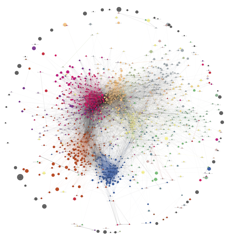
It is worth noting another property L-Spar, which we used with might and main: improving the readability of the picture. Due to the dramatic reduction in the number of edges, it may now be possible to better visualize the Hair Spheres of social networks and show communities on them. An example of such visualization was given in the previous part of this post, where there was a graph from 1285 web domains after the application of L-Spar and before it.

Select the number of clusters

One of the problems of k-medoids is a fixed number of clusters. To find the optimal number of clusters, we tried several options. The trouble with modularity, conductivity, normalized cut and other metrics is that they suffer from a resolution limit, and their maximum is reached at too low (compared to what our eyes tell us). Here, for example, the modularity graph, obtained by us depending on for the graph of web domains from 1029 nodes more than a year ago:



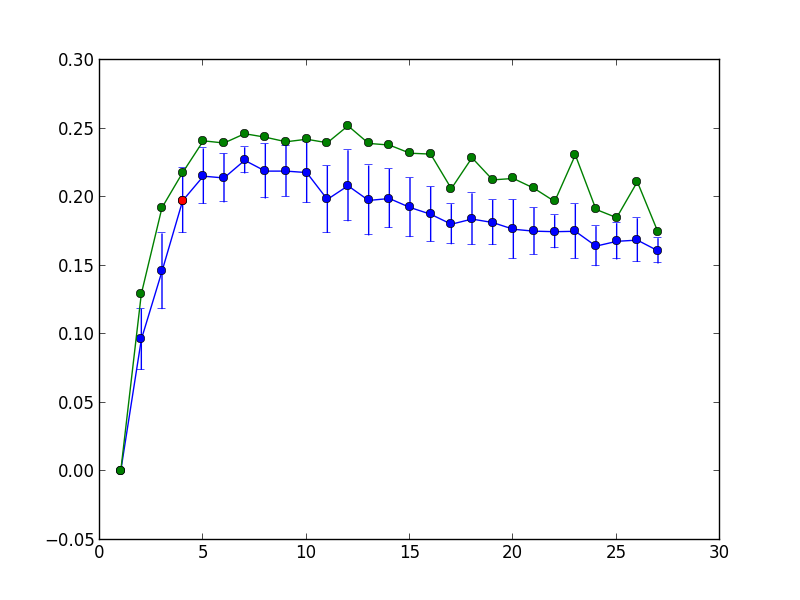
The blue color shows the average modularity and its 1.95 standard deviations per 100 repetitions of the k-medoids, while green shows the maximum modularity per 100 repetitions. The point corresponding to the maximum number of clusters is highlighted in red. at which the average modularity is not lower than the upper limit of the confidence interval at . Point is already in the zone of falling modularity, whereas approximately as many communities are present in the data, as it seems visually (WTF). Exactly in the end it was chosen.

Stable cores

The modifications described above may be good in terms of scalability, but they lead to two interesting problems. Firstly, the quality of clusters may fall: it is not obvious how much the logicality of the partitioning falls when the heuristics are simplified (especially when a subgraph is selected or most of the edges are removed). Secondly, the stability of the result is under threat: splitting into clusters at the second run will differ significantly from splitting at the first, even with the same initial data. All our modifications even more randomized the algorithm. And what if the graph also evolves over time? How to identify with each other clusters from different runs?



We conducted a small experiment with a domain graph of 1209 nodes to check the stability of the k-medoids. For two different runs of the algorithm with all modifications, we found the most “central” nodes (by the harmonic centrality metric) within each cluster — a quarter of the total number of nodes in the cluster, but no less than eight. Then for each cluster from the first partition we found a cluster of the second partition, which includes the largest number of its “central” nodes. If a then for the majority of pairs of partitions only for 9-10 clusters from the first run it is possible to find an analogue from the second, where at least half of the “central nodes” coincide. This is clearly not enough for, for example, building segments for advertising campaigns. At the same time, it is not known what result would have taken place in dynamics, since over time, both the popularity of domains and their connections change.



Articles are devoted to this problem: one , two , three . They say that adding or removing only one vertex can radically change the whole partition, affecting not only the nearest neighbors, but also the remote parts of the graph. One solution to this problem is clustering averaging. This is an attempt to adapt the ensemble approach, well-proven in training with the teacher, for clustering problems. If you do not one, but, say, 100 runs of the algorithm, and then find groups of vertices (cores) that always fall together in the same cluster, then these groups will be much more stable in time than the results of individual runs. The only drawback of this method is speed: dozens of repetitions can negate the achievements of the acceleration of the algorithm. However, when nuclei are found, it is possible to sample the graph with smaller losses, i.e. use clara.



We have implemented a slightly different option for obtaining cores. For each pair of vertices, we consider in what proportion of the runs they fall into the same cluster. The data obtained can be interpreted as the weight of the ribs (degree of proximity) in the new, complete graph. Further on this graph hierarchical clustering is built. We used the agglomerative method scipy.linkage and the Ward method as a function of distance when merging clusters.



Here you can look at the full version of the dendrogram.



The cut-off threshold can be set at any height, while obtaining a different number of clusters. It may seem the most logical to set such a threshold that the number of clusters is equal to the number of clusters in each k-medoids run when receiving the dendrogram itself. However, in practice, oddly enough, if for k-medoids to pick the right , then at lowering the threshold on the dendrogram it is possible to allocate logical “subcommunities” of a much smaller size. For example, in the part of the tree below, a turquoise cluster was obtained at a threshold corresponding to 12 cores, while at lower threshold this cluster could be split into 2 meaningful subclusters: cars from above and psychology from below. Here is a screenshot:





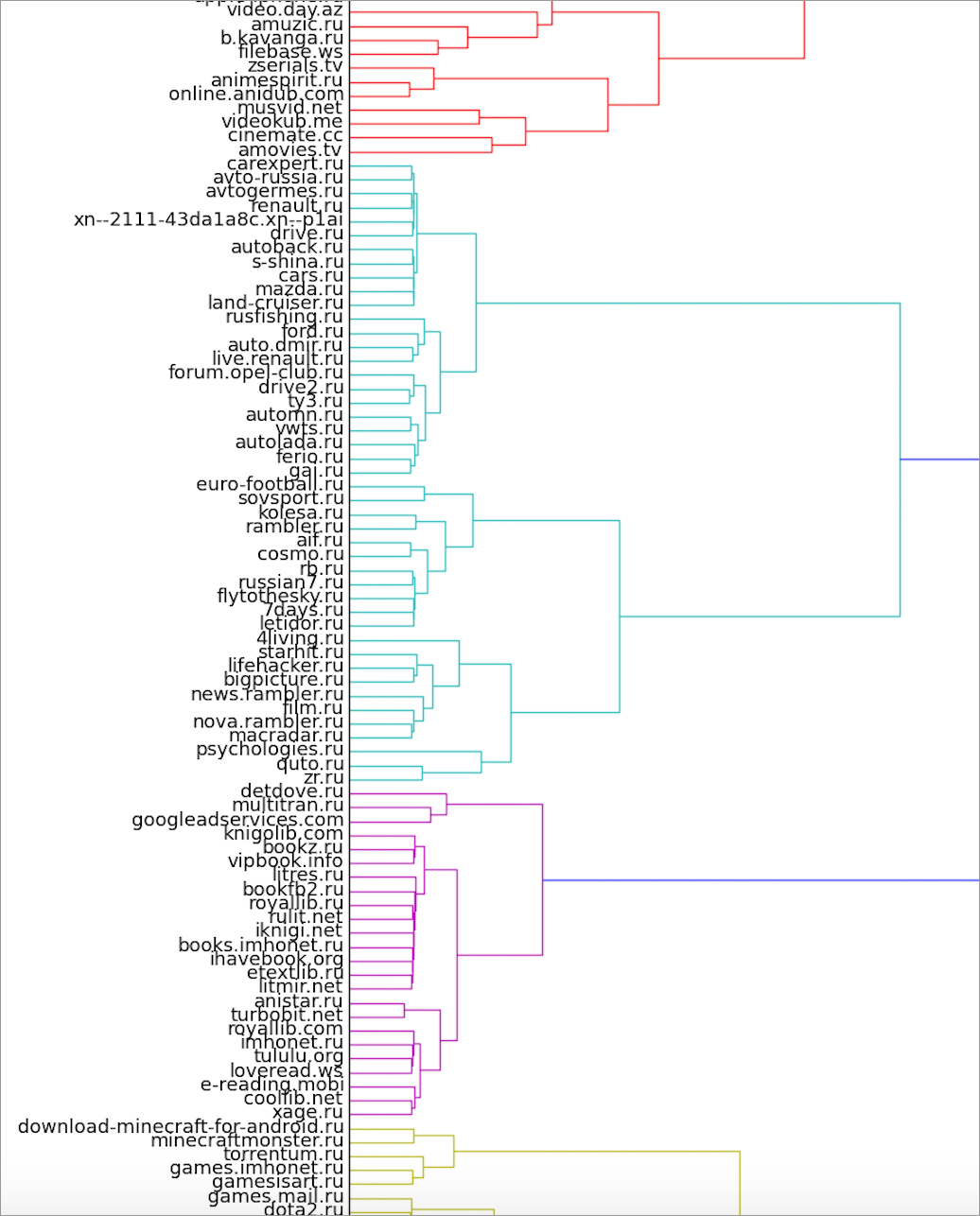
The frame also includes a cluster of books and pieces of game and serial clusters.



The domain cores obtained by this method successfully function as user segments in our Exebid.DCA RTB system.



There are already several excellent algorithms for allocating communities, faster and more efficiently than our practices. Louvain, MLR-MCL, SCD, Infomap, Spinner, Stochastic Blockmodeling are some of them. In the future we plan to write about our experiments with these methods. But we wanted to write something ourselves. Here are some of the areas for improvement:

• The calculation of the Jacquard measure is the most resource-intensive step requiring operations. Known fast approximate method of obtaining similarities called MinHash. You can read about it, for example, here . There are still more complex methods, for example, BayesLSH.
  
  
  
  
• Computational complexity, depending on the number of clusters, this feature of the k-medoids makes it inapplicable for a wide range of tasks. It can be dealt with this way: for each medoid, at each iteration, find and save a list of “neighboring” medoids, and only recalculate them at each iteration.
  
  
  
  
• The arbitrariness of the choice of the number of clusters - Another difficulty with k-medoids. One of the outputs is to find a standing metric by which to compare the results for different . This role is claimed by the WCC (Weighted Community Clustering coefficient), based on the analysis of closed triangles inside and outside the clusters. It is possible that the choice of the optimal replacement at each iteration should be transferred to this metric.

Thanks for attention!