Contingency Tables: Log Linear Models and Markov Networks
In the previous part of the publication, the method of factorization of non-negative matrices was considered as a reduction of dimension and visualization of contingency tables. In this part a statistical analysis of the obtained diagrams will be carried out using log-linear models. I will remind, examples are shown for complex survey data - stratified, clustered and weighted samples. This circumstance implies the use of special methods for evaluating and selecting models. Markov networks are used to visualize the results obtained. This is a convenient tool for graphical representation of the interaction of factors of log-linear models.

')
Briefly about the previous series. According to the ESS data for 2012, a table was drawn up for the general population “Men aged 25-40 years” on the degree of support for human values in each of the survey countries. To reduce the dimension of the representation of the matrix of size 29x21, defined by the table, NMF transformation of rank 5 was made. I repeat the final positioning map of all 29 countries in the resulting space so that it is in front of you

Formulation of the problem
The constructed map suggests between which countries (or clusters of countries) the hypothesis about the independence of the distribution of shares of value variables from countries (clusters of countries) can be rejected. It is required to statistically confirm the emerging hypotheses. For examples we will use the following groups of countries
Of course, the choice is not limited to these examples, and the researcher can choose those countries or clusters of countries that coincide with his interests.
In addition to testing hypotheses, the question arises - how do value factors interact depending on the group of selected countries? It is required to reveal these possible differences.
Some words about contingency tables.
All value variables in the table for performing NMF transformation were perceived as one variable with multiple choice (multiple response variable). It was necessary to present the data in the form of a two-dimensional table, that is, a table formed by two variables. In reality, our situation is somewhat different, a complete set of 21 value variables and 1 variable indicating a country define a 22-dimensional contingency table.
This will probably seem surprising, but from the point of view of building statistical models, multidimensional contingency tables (with single response variables and no missing answers) are a simpler situation than tables with multiple response variables. In addition, using NMF, the dimension of the table was reduced to 6 - 5 latent variables + 1 variable with the country.
Log Linear Models
The classic method for analyzing a multidimensional contingency table is the construction of its log-linear model. Log-linear analysis can be interpreted as a generalization of the chi-square test for the case of multidimensional tables. The definition of log-linear models can be viewed in Wikipedia (eng). On this topic materials are available with examples in Russian, for example, here or here , as well as detailed lectures in English here .
Before turning to calculations, we note that in the general case, multidimensional contingency tables determine the multinomial distribution . But when the marginal sums of this distribution in one dimension or several dimensions are fixed, we get the so-called product-multinomial distribution . Therefore, it is required to impose additional restrictions on the parameters of log-linear models for such tables. Details can be found in chapter 12 of the book [1]. In our case, the marginal sums are fixed in one dimension - the size of the general sets in each of the countries are constants. This means that the main effect corresponding to a country variable cannot be excluded from the model.
Last note. We will omit the question of which tables for survey data are considered sparse and, as a result, we will not conduct the appropriate checks.
Identify and compare models
We still use the survey [2] package of the R environment to account for the effects of stratification, clustering, and sample weighting. In more detail about it it was reported in one of the last publications . The parameters of the log-linear models for complex survey data are exactly the same as for the tables without considering the study design. Correction of formulas for calculating the significance of model parameters (both individually and in aggregate) is required.
Example 1 , the simplest - a table for Russia and Slovakia with one latent variable “money | success. "

We build two models: implying the independence of factors and saturated.
that a saturated model is not significantly better than an independent model.
That is, we cannot reject the null hypothesis of independence of variables in the table.
For comparison, this is a table with the results of an independent model.

Example 2. Consider a table with all five latent variables for France and Russia.
The log-linear model, which assumes the pairwise independence of all factors is rejected. A model with all the elements of the second order is acceptable. This model can (and should) be simplified - by the results of the wald and likelihood ratio of criteria, the second-order parameters for the variable defining the country and the last two latent variables of the heatmap are discarded.
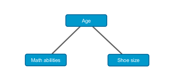
Conditional independence. Why are mathematical skills and shoe size dependent factors?
This variation is on a classic example. Suppose the respondent’s mathematical abilities are determined by the following gradation — high, medium, or low. We are constructing a contingency table with these two variables, for example, for the population of the whole of Russia. The hypothesis of independence of these variables can be boldly rejected. People with a large shoe size have higher mathematical ability. What is the reason? In the absence of a hidden variable - age. It is clear that, up to a certain point, age correlates positively with both mathematical abilities and shoe size. If we fix the age ( Age = k ), then for any k the table of joint distribution of the values M (mat. Abilities) and S (shoe size) will not indicate the presence of a significant relationship between them. In this case, it is said that the quantities M and S are conditionally independent. This result is naturally expressed in the form of a Markov network — an undirected graphical model.
I will add that on Habré there is an excellent article about Bayesian networks - directed graphic models.
Graphic representation of log linear models
The previous example can be generalized and extended to arbitrary hierarchical log-linear models, which was implemented in [3]. Consider a number of possible options for the three variables A , B and C.
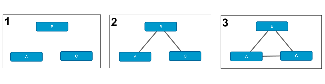
These Markov networks correspond to the following log-linear models.
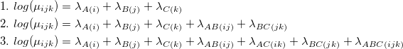
Note that not every hierarchical log-linear model can be represented as a Markov network. For example - model AB / AC / BC . But any model can be uniquely embedded in the minimal Markov network. Details of the correspondence between log-linear and graphical models can be found in the book [1] or article [3].
Final results
Markov networks make it relatively easy to navigate the relationship of variables and compare the results of different tables.


We see that in the case of Russia and Slovakia there is a significant relationship between the country and the variable “the search for adventure is important and the risk or opportunity to have fun.” With other values, the Country variable is conditionally independent.
Whereas in France and Russia there is a significant difference in relation to the three statements: “it is important to be rich or be successful”, “it is important to have a good time” and “it is important to be simple and modest”.
Both of these conclusions are consistent with the results of the heatmap.
As for the relationship between latent variables, the graphs for these pairs of countries differ by only one edge. For Russia and Slovakia, the variables “it is important to have a good time” and “it is important to follow the rules or it is important to help others” are conditionally independent.
In conclusion, I note that in log-linear models for complex survey data, a step-by-step model selection based on AIC or BIC results has not yet been implemented. Articles with the adaptation of these criteria to such data began to appear only in recent years. In particular, this year an article [4] was published, one of whose co-authors is T. Lumley, the creator of the survey package.
Literature:
[1] G. Tutz (2011) Regression for Categorical Data, Cambridge University Press.
[2] T. Lumley (2014) survey: analysis of complex survey samples. R package version 3.30.
[3] JN Darroch, SL Lauritzen, and TP Speed (1980) Markov fields and log-linear interaction models for contingency tables. Annals of Statistics 8 (3), 522–539.
[4] T. Lumley, A. Scott (2015) AIC and BIC for modeling with complex survey data, J. Surv. Stat. Method. 3 (1), 1-18.
')
Briefly about the previous series. According to the ESS data for 2012, a table was drawn up for the general population “Men aged 25-40 years” on the degree of support for human values in each of the survey countries. To reduce the dimension of the representation of the matrix of size 29x21, defined by the table, NMF transformation of rank 5 was made. I repeat the final positioning map of all 29 countries in the resulting space so that it is in front of you
Formulation of the problem
The constructed map suggests between which countries (or clusters of countries) the hypothesis about the independence of the distribution of shares of value variables from countries (clusters of countries) can be rejected. It is required to statistically confirm the emerging hypotheses. For examples we will use the following groups of countries
- Russia and Slovakia, according to the results of hierarchical clustering - neighbors;
- France and Russia, as variants of countries with different views.
Of course, the choice is not limited to these examples, and the researcher can choose those countries or clusters of countries that coincide with his interests.
In addition to testing hypotheses, the question arises - how do value factors interact depending on the group of selected countries? It is required to reveal these possible differences.
Some words about contingency tables.
All value variables in the table for performing NMF transformation were perceived as one variable with multiple choice (multiple response variable). It was necessary to present the data in the form of a two-dimensional table, that is, a table formed by two variables. In reality, our situation is somewhat different, a complete set of 21 value variables and 1 variable indicating a country define a 22-dimensional contingency table.
This will probably seem surprising, but from the point of view of building statistical models, multidimensional contingency tables (with single response variables and no missing answers) are a simpler situation than tables with multiple response variables. In addition, using NMF, the dimension of the table was reduced to 6 - 5 latent variables + 1 variable with the country.
Log Linear Models
The classic method for analyzing a multidimensional contingency table is the construction of its log-linear model. Log-linear analysis can be interpreted as a generalization of the chi-square test for the case of multidimensional tables. The definition of log-linear models can be viewed in Wikipedia (eng). On this topic materials are available with examples in Russian, for example, here or here , as well as detailed lectures in English here .
Before turning to calculations, we note that in the general case, multidimensional contingency tables determine the multinomial distribution . But when the marginal sums of this distribution in one dimension or several dimensions are fixed, we get the so-called product-multinomial distribution . Therefore, it is required to impose additional restrictions on the parameters of log-linear models for such tables. Details can be found in chapter 12 of the book [1]. In our case, the marginal sums are fixed in one dimension - the size of the general sets in each of the countries are constants. This means that the main effect corresponding to a country variable cannot be excluded from the model.
Last note. We will omit the question of which tables for survey data are considered sparse and, as a result, we will not conduct the appropriate checks.
Identify and compare models
We still use the survey [2] package of the R environment to account for the effects of stratification, clustering, and sample weighting. In more detail about it it was reported in one of the last publications . The parameters of the log-linear models for complex survey data are exactly the same as for the tables without considering the study design. Correction of formulas for calculating the significance of model parameters (both individually and in aggregate) is required.
Load the data, select the gene. aggregate, add latent variables to the database and set the study design.
library(foreign) library(data.table) library(survey) srv.data <- read.dta("ESS6e02_1.dta") srv.variables <- data.table(name = names(srv.data), title = attr(srv.data, "var.labels")) srv.data <- data.table(srv.data) setkey(srv.data, cntry) setkey(srv.variables, name) fr.dt<-data.table(read.dta("ESS6_FR_SDDF.dta")) ru.dt<-data.table(read.dta("ESS6_RU_SDDF.dta")) ru.dt[,psu:=psu+150] # psu values are changed to avoid their intersections between countries sk.dt<-data.table(read.dta("ESS6_SK_SDDF.dta")) sddf.data <- rbind(fr.dt, ru.dt, sk.dt) setkey(sddf.data, cntry, idno) cntries.data <- srv.data[J(c("FR", "RU", "SK"))] cntries.data[ ,weight:=dweight*pweight] setkey(cntries.data, cntry, idno ) cntries.data <- cntries.data[sddf.data] cntries.data <- cntries.data[gndr == 'Male' & agea >= 25 & agea<=40, ] # add the latent variables<b> a.1, a.2, ..., a.5</b> to the cntries.data answers <- c('Very much like me', 'Like me') cntries.data[,a.1:= imprich %in% answers | ipsuces %in% answers] cntries.data[,a.2:= ipgdtim %in% answers] cntries.data[,a.3:= ipmodst %in% answers] cntries.data[,a.4:= ipadvnt %in% answers | impfun %in% answers] cntries.data[,a.5:= ipfrule %in% answers | ipudrst %in% answers] # define survey design srv.design.data <- svydesign(ids = ~psu, strata = ~stratify, weights = ~weight, data = cntries.data) options(survey.lonely.psu="adjust") Example 1 , the simplest - a table for Russia and Slovakia with one latent variable “money | success. "
We build two models: implying the independence of factors and saturated.
Calculations show ...
Analysis of Deviance Table
Model 1: y ~ a.1 + cntry
Model 2: y ~ a.1 + cntry + a.1: cntry
Deviance = 0.1240613 p = 0.4737981
Score = 0.1217862 p = 0.4778766
ru.sk.data <- subset(srv.design.data, cntry %in% c("RU", "SK")) srv.loglin.model.ind <- svyloglin(~a.1+cntry, ru.sk.data) srv.loglin.model.sq <- update(srv.loglin.model.ind, ~.^2) anova(srv.loglin.model.ind, srv.loglin.model.sq) Analysis of Deviance Table
Model 1: y ~ a.1 + cntry
Model 2: y ~ a.1 + cntry + a.1: cntry
Deviance = 0.1240613 p = 0.4737981
Score = 0.1217862 p = 0.4778766
that a saturated model is not significantly better than an independent model.
That is, we cannot reject the null hypothesis of independence of variables in the table.
For comparison, this is a table with the results of an independent model.
Example 2. Consider a table with all five latent variables for France and Russia.
The log-linear model, which assumes the pairwise independence of all factors is rejected. A model with all the elements of the second order is acceptable. This model can (and should) be simplified - by the results of the wald and likelihood ratio of criteria, the second-order parameters for the variable defining the country and the last two latent variables of the heatmap are discarded.
Calculations
cntry: a.1 cntry: a.2 cntry: a.3 cntry: a.4 cntry: a.5
0.000 0.000 0.000 0.437 0.524
0.6066181
fr.ru.data <- subset(srv.design.data, cntry %in% c("FR", "RU")) srv.loglin.model.ind <- svyloglin(~ a.1 + a.2 + a.3 + a.4 + a.5 + cntry, fr.ru.data) srv.loglin.model.sq <- update(srv.loglin.model.ind, ~.^2) srv.loglin.model.tri <- update(srv.loglin.model.ind, ~.^3) srv.loglin.model.four <- update(srv.loglin.model.ind, ~.^4) anova(srv.loglin.model.ind, srv.loglin.model.sq)$dev$p[3] #5.745843e-50 c( anova(srv.loglin.model.sq, srv.loglin.model.tri), anova(srv.loglin.model.sq, srv.loglin.model.four) ) # 0.7335668 0.7427429 sapply(paste('cntry:a.',1:5,sep=""), function(x) round(regTermTest(srv.loglin.model.sq, x)$p, 3) ) cntry: a.1 cntry: a.2 cntry: a.3 cntry: a.4 cntry: a.5
0.000 0.000 0.000 0.437 0.524
anova(update(srv.loglin.model.sq, ~. -cntry:(a.4 + a.5)), srv.loglin.model.sq)$dev$p[3] 0.6066181
Conditional independence. Why are mathematical skills and shoe size dependent factors?
This variation is on a classic example. Suppose the respondent’s mathematical abilities are determined by the following gradation — high, medium, or low. We are constructing a contingency table with these two variables, for example, for the population of the whole of Russia. The hypothesis of independence of these variables can be boldly rejected. People with a large shoe size have higher mathematical ability. What is the reason? In the absence of a hidden variable - age. It is clear that, up to a certain point, age correlates positively with both mathematical abilities and shoe size. If we fix the age ( Age = k ), then for any k the table of joint distribution of the values M (mat. Abilities) and S (shoe size) will not indicate the presence of a significant relationship between them. In this case, it is said that the quantities M and S are conditionally independent. This result is naturally expressed in the form of a Markov network — an undirected graphical model.
I will add that on Habré there is an excellent article about Bayesian networks - directed graphic models.
Graphic representation of log linear models
The previous example can be generalized and extended to arbitrary hierarchical log-linear models, which was implemented in [3]. Consider a number of possible options for the three variables A , B and C.
These Markov networks correspond to the following log-linear models.
Note that not every hierarchical log-linear model can be represented as a Markov network. For example - model AB / AC / BC . But any model can be uniquely embedded in the minimal Markov network. Details of the correspondence between log-linear and graphical models can be found in the book [1] or article [3].
Final results
Markov networks make it relatively easy to navigate the relationship of variables and compare the results of different tables.
We see that in the case of Russia and Slovakia there is a significant relationship between the country and the variable “the search for adventure is important and the risk or opportunity to have fun.” With other values, the Country variable is conditionally independent.
Whereas in France and Russia there is a significant difference in relation to the three statements: “it is important to be rich or be successful”, “it is important to have a good time” and “it is important to be simple and modest”.
Both of these conclusions are consistent with the results of the heatmap.
As for the relationship between latent variables, the graphs for these pairs of countries differ by only one edge. For Russia and Slovakia, the variables “it is important to have a good time” and “it is important to follow the rules or it is important to help others” are conditionally independent.
In conclusion, I note that in log-linear models for complex survey data, a step-by-step model selection based on AIC or BIC results has not yet been implemented. Articles with the adaptation of these criteria to such data began to appear only in recent years. In particular, this year an article [4] was published, one of whose co-authors is T. Lumley, the creator of the survey package.
Literature:
[1] G. Tutz (2011) Regression for Categorical Data, Cambridge University Press.
[2] T. Lumley (2014) survey: analysis of complex survey samples. R package version 3.30.
[3] JN Darroch, SL Lauritzen, and TP Speed (1980) Markov fields and log-linear interaction models for contingency tables. Annals of Statistics 8 (3), 522–539.
[4] T. Lumley, A. Scott (2015) AIC and BIC for modeling with complex survey data, J. Surv. Stat. Method. 3 (1), 1-18.
Source: https://habr.com/ru/post/264801/
All Articles