Introduction to machine learning with scikit-learn (translation of documentation)
This article is a translation of the introduction to machine learning, presented on the official website scikit-learn .
In this part we will talk about the terms of machine learning that we use to work with scikit-learn, and give a simple example of learning.
In general, the problem of machine learning is reduced to obtaining a set of data samples and, subsequently, to attempts to predict the properties of unknown data. If each data set is not a single number, but, for example, a multidimensional entity (multi-dimensional entry or multivariate data), then it should have several features or features.
')
Machine learning can be divided into several large categories:
Machine learning is learning how to isolate certain properties of a data sample and apply them to new data. That is why the common practice of evaluating an algorithm in Machine Learning is to manually split the data into two data sets. The first of these is the training sample, and the properties of the data are studied on it. The second is a control sample , these properties are tested on it.
Scikit-learn is set together with several standard data samples, for example, iris and digits for classification, and boston house prices dataset for regression analysis.
Next, we run the Python interpreter from the command line and load the iris and digits samples. Let's set the following conventions: $ means starting the Python interpreter, and >>> means starting the Python command line:
A data set is a dictionary object that contains all the data and some metadata about it. This data is stored with a .data extension, for example, n_samples, n_features arrays. In machine learning with a teacher, one or more dependent variables are stored with the .target extension. For more information on datasets, go to the appropriate section .
For example, the digits.data dataset provides access to features that can be used to classify numeric samples:
and digits.target makes it possible to determine in a numerical sample, which digit corresponds to each numerical representation, which we will study:
Usually, the data is presented in the form of a two-dimensional array, n_samples, n_features have such a shape, although the source data may have a different shape. In the case of numbers, each source sample is a representation of the form (8, 8), which can be accessed using:
The following simple example with this data set illustrates how, based on the task, you can generate data for use in scikit-learn.
In the case of a numeric data set, the goal of learning is to predict, taking into account the data representation, which digit is shown. We have samples of each of the ten possible classes (numbers from 0 to 9) in which we train the estimator (estimator) so that it can predict the class to which the unlabeled sample belongs.
In scikit-learn, the estimation algorithm for a classifier is a Python object that executes the fit (X, y) and predict (T) methods. An example of an estimation algorithm is the class sklearn.svm.SVC performs the classification by the support vector machine. The designer of the estimation algorithm accepts model parameters as arguments, but to reduce the time, we will consider this algorithm as a black box:
In this example, we set the value of gamma manually. You can also automatically determine the appropriate values for the parameters using tools such as grid search and cross validation .
We called an instance of our clf evaluation algorithm, since it is a classifier. Now it should be applied to the model, i.e. he must learn on the model. This is done by running our training sample through the fit method. As a training sample, we can use all the representations of our data, except the last. We made this sample using the Python syntax [: -1], which created a new array containing all but the last entity from digits.data:
Now we can predict new values, in particular, we can ask the classifier what number is contained in the last representation in the digits data set, which we did not use in the classifier training:
The corresponding image is presented below:
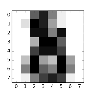
As you can see, this is a difficult task: the presentation is in poor resolution. Do you agree with the classifier?
The complete solution to this classification problem is available as an example, which you can run and study: Recognizing hand-written digits .
In scikit, the model can be saved using a built-in module called pickle :
In the particular case of scikit, it may be more useful to notice pickle on the joblib library (joblib.dump & joblib.load), which is more efficient for working with large amounts of data, but it allows you to save the model only on disk, and not in the line:
Then you can load the saved model (possibly in another Python process) with:
Note that joblib.dump returns a list of file names. Each individual numpy array contained in the clf object is parsed as a separate file in the file system. All files must be in the same folder when you load the model again with joblib.load.
Please note that pickle has some security and maintenance issues. For more detailed information on model storage in scikit-learn, refer to the Model persistence section.
In this part we will talk about the terms of machine learning that we use to work with scikit-learn, and give a simple example of learning.
Machine learning: posing the question
In general, the problem of machine learning is reduced to obtaining a set of data samples and, subsequently, to attempts to predict the properties of unknown data. If each data set is not a single number, but, for example, a multidimensional entity (multi-dimensional entry or multivariate data), then it should have several features or features.
')
Machine learning can be divided into several large categories:
- learning with a teacher (or guided learning). Here the data are presented along with additional features that we want to predict. ( Click here to go to the Scikit-Learn Training with Teacher page). This can be any of the following tasks:
- classification : data samples belong to two or more classes and we want to learn from the already marked data to predict the class of unlabeled samples. An example of a classification problem is handwriting recognition, the purpose of which is to assign each of the input data sets one of a finite number of discrete categories. Another way to understand classification is to understand it as a discrete (as opposed to continuous) form of managed learning, where we have a limited number of categories provided for N samples; and we try to mark them with the correct category or class.
- regression analysis : if the desired output consists of one or more continuous variables, then we are faced with a regression analysis. An example of solving such a problem is the prediction of the length of a salmon as a result of a function of its age and weight.
- learning without a teacher (or self-study). In this case, the training sample consists of a set of input data X without any corresponding values. The purpose of such tasks may be to determine groups of similar elements within the data. This is called clustering or cluster analysis. Also, the task may be to establish the distribution of data within the input space, called density density ( density estimation ). Or it could be the extraction of data from a high dimensional space into a two-dimensional or three-dimensional space in order to visualize the data. ( Click here to go to the Scikit-Learn tuition without a teacher.)
Training Sample and Control Sampling
Machine learning is learning how to isolate certain properties of a data sample and apply them to new data. That is why the common practice of evaluating an algorithm in Machine Learning is to manually split the data into two data sets. The first of these is the training sample, and the properties of the data are studied on it. The second is a control sample , these properties are tested on it.
Sample load
Scikit-learn is set together with several standard data samples, for example, iris and digits for classification, and boston house prices dataset for regression analysis.
Next, we run the Python interpreter from the command line and load the iris and digits samples. Let's set the following conventions: $ means starting the Python interpreter, and >>> means starting the Python command line:
$ python >>> from sklearn import datasets >>> iris = datasets.load_iris() >>> digits = datasets.load_digits() A data set is a dictionary object that contains all the data and some metadata about it. This data is stored with a .data extension, for example, n_samples, n_features arrays. In machine learning with a teacher, one or more dependent variables are stored with the .target extension. For more information on datasets, go to the appropriate section .
For example, the digits.data dataset provides access to features that can be used to classify numeric samples:
>>> print(digits.data) [[ 0. 0. 5. ..., 0. 0. 0.] [ 0. 0. 0. ..., 10. 0. 0.] [ 0. 0. 0. ..., 16. 9. 0.] ..., [ 0. 0. 1. ..., 6. 0. 0.] [ 0. 0. 2. ..., 12. 0. 0.] [ 0. 0. 10. ..., 12. 1. 0.]] and digits.target makes it possible to determine in a numerical sample, which digit corresponds to each numerical representation, which we will study:
>>> digits.target array([0, 1, 2, ..., 8, 9, 8]) Dataset form
Usually, the data is presented in the form of a two-dimensional array, n_samples, n_features have such a shape, although the source data may have a different shape. In the case of numbers, each source sample is a representation of the form (8, 8), which can be accessed using:
>>> digits.images[0] array([[ 0., 0., 5., 13., 9., 1., 0., 0.], [ 0., 0., 13., 15., 10., 15., 5., 0.], [ 0., 3., 15., 2., 0., 11., 8., 0.], [ 0., 4., 12., 0., 0., 8., 8., 0.], [ 0., 5., 8., 0., 0., 9., 8., 0.], [ 0., 4., 11., 0., 1., 12., 7., 0.], [ 0., 2., 14., 5., 10., 12., 0., 0.], [ 0., 0., 6., 13., 10., 0., 0., 0.]]) The following simple example with this data set illustrates how, based on the task, you can generate data for use in scikit-learn.
Training and Forecasting
In the case of a numeric data set, the goal of learning is to predict, taking into account the data representation, which digit is shown. We have samples of each of the ten possible classes (numbers from 0 to 9) in which we train the estimator (estimator) so that it can predict the class to which the unlabeled sample belongs.
In scikit-learn, the estimation algorithm for a classifier is a Python object that executes the fit (X, y) and predict (T) methods. An example of an estimation algorithm is the class sklearn.svm.SVC performs the classification by the support vector machine. The designer of the estimation algorithm accepts model parameters as arguments, but to reduce the time, we will consider this algorithm as a black box:
>>> from sklearn import svm >>> clf = svm.SVC(gamma=0.001, C=100.) Selection of parameters for the model
In this example, we set the value of gamma manually. You can also automatically determine the appropriate values for the parameters using tools such as grid search and cross validation .
We called an instance of our clf evaluation algorithm, since it is a classifier. Now it should be applied to the model, i.e. he must learn on the model. This is done by running our training sample through the fit method. As a training sample, we can use all the representations of our data, except the last. We made this sample using the Python syntax [: -1], which created a new array containing all but the last entity from digits.data:
>>> clf.fit(digits.data[:-1], digits.target[:-1]) SVC(C=100.0, cache_size=200, class_weight=None, coef0=0.0, degree=3, gamma=0.001, kernel='rbf', max_iter=-1, probability=False, random_state=None, shrinking=True, tol=0.001, verbose=False) Now we can predict new values, in particular, we can ask the classifier what number is contained in the last representation in the digits data set, which we did not use in the classifier training:
>>> clf.predict(digits.data[-1]) array([8]) The corresponding image is presented below:
As you can see, this is a difficult task: the presentation is in poor resolution. Do you agree with the classifier?
The complete solution to this classification problem is available as an example, which you can run and study: Recognizing hand-written digits .
Saving model
In scikit, the model can be saved using a built-in module called pickle :
>>> from sklearn import svm >>> from sklearn import datasets >>> clf = svm.SVC() >>> iris = datasets.load_iris() >>> X, y = iris.data, iris.target >>> clf.fit(X, y) SVC(C=1.0, cache_size=200, class_weight=None, coef0=0.0, degree=3, gamma=0.0, kernel='rbf', max_iter=-1, probability=False, random_state=None, shrinking=True, tol=0.001, verbose=False) >>> import pickle >>> s = pickle.dumps(clf) >>> clf2 = pickle.loads(s) >>> clf2.predict(X[0]) array([0]) >>> y[0] 0 In the particular case of scikit, it may be more useful to notice pickle on the joblib library (joblib.dump & joblib.load), which is more efficient for working with large amounts of data, but it allows you to save the model only on disk, and not in the line:
>>> from sklearn.externals import joblib >>> joblib.dump(clf, 'filename.pkl') Then you can load the saved model (possibly in another Python process) with:
>>> clf = joblib.load('filename.pkl') Note that joblib.dump returns a list of file names. Each individual numpy array contained in the clf object is parsed as a separate file in the file system. All files must be in the same folder when you load the model again with joblib.load.
Please note that pickle has some security and maintenance issues. For more detailed information on model storage in scikit-learn, refer to the Model persistence section.
Source: https://habr.com/ru/post/264241/
All Articles