Interpolation of data: we connect points so that it was beautiful
How to build a graph for n points? The simplest thing is to mark them with markers on the coordinate grid. However, for clarity, they want to connect to get an easily readable line. The easiest way to connect the points is by straight lines. But the graph-line is quite difficult to read: the look clings to the corners, and does not slide along the line. Yes, and look kinks are not very beautiful. It turns out that in addition to broken lines, you need to be able to build curves. However, you need to be careful not to get this:
Recovery of intermediate values of a function, which in this case is given in tabular form as points P 1 ... P n , is called interpolation. There are many interpolation methods, but all of them can be reduced to finding the n - 1 function to calculate intermediate points on the corresponding segments. In this case, the given points must be computable through the corresponding functions. Based on this, a graph can be built:
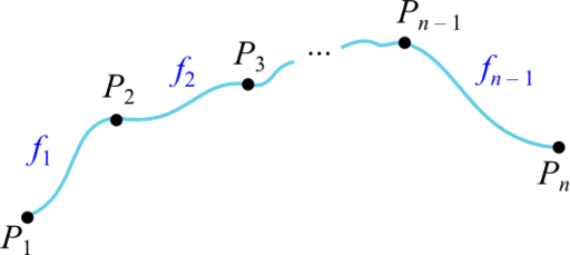
The functions f i can be very different, but most often they use polynomials of some degree. In this case, the final interpolating function (piecewise defined on the intervals bounded by points P i ) is called a spline .
')
In different graphing tools — editors and libraries — the problem of “beautiful interpolation” is solved differently. At the end of the article there will be a small overview of the existing options. Why at the end? So that after a number of the above calculations and reflections it was possible to guess which of the "serious guys" use what methods.
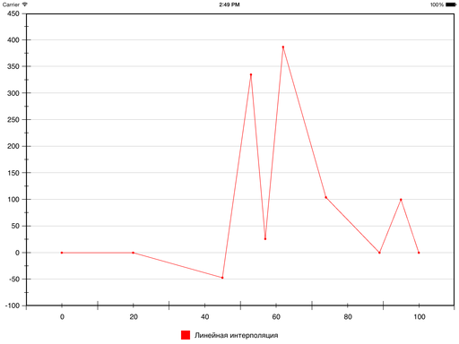
The simplest example is linear interpolation, in which polynomials of the first degree are used, and as a result we get a polyline connecting the given points.
Let's add some specifics. Here is a set of points (taken almost from the ceiling):
The result of linear interpolation of these points is as follows:
However, as noted above, sometimes you want to end up with a smooth curve.
What is smoothness? Household answer: no sharp corners. Mathematical: continuity of derivatives. Moreover, in mathematics, smoothness has an order equal to the number of the last continuous derivative, and the area on which this continuity is preserved. That is, if the function has a smoothness of order 1 on the segment [ a ; b ], this means that on [ a ; b ] it has a continuous first derivative, but the second derivative already suffers a gap at some points.
A spline in the context of smoothness is the concept of a defect. A spline defect is the difference between its degree and its smoothness. The degree of the spline is the maximum degree of the polynomials used in it.
It is important to note that the “dangerous” points of the spline (at which smoothness can be broken) are just P i , that is, the junction points of the segments at which the transition from one polynomial to another occurs. All other points are “safe”, because a polynom on the domain of its definition has no problems with the continuity of derivatives.
In order to achieve smooth interpolation, it is necessary to increase the degree of polynomials and choose their coefficients so that the continuity of the derivatives is preserved at the boundary points.
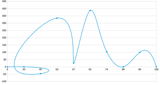
Traditionally, to solve this problem, polynomials of the third degree are used and the continuity of the first and second derivatives is achieved. What turns out is called the cubic spline of defect 1 . Here is how it looks for our data:

The curve is really smooth. But if we assume that this is a schedule of some process or phenomenon that needs to be shown to an interested person, then this method is most likely not suitable. The problem is in false extremes. They appeared due to too much curvature, which was intended to ensure the smoothness of the interpolation function. But this behavior is not at all useful to the viewer, because he is deceived about the peak values of the function. And for the sake of visual visualization of these values, in fact, everything was started.
So you need to look for other solutions.
Another traditional solution, except for cubic splines of defect 1, is Lagrange polynomials. These are polynomials of degree n - 1 that take given values at given points. That is, division into segments does not occur here; the entire sequence is described by one polynomial.
But what happens is:
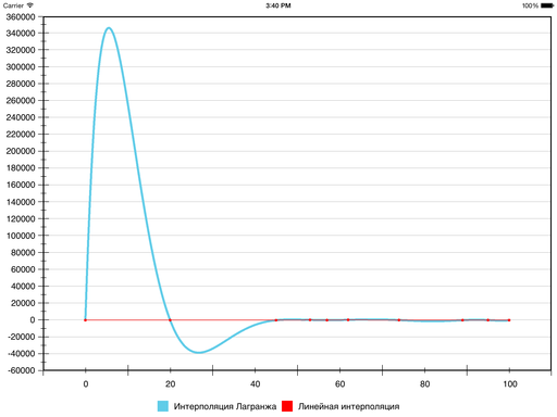
Smoothness, of course, is present, but visibility has suffered so much that ... perhaps I should look for other methods. On some data sets, the result is normal, but in general, the error with respect to linear interpolation (and, accordingly, false extremes) may be too large - due to the fact that there is only one polynomial for all segments.
In computer graphics, Bezier curves , represented by kth- degree polynomials, are very widely used.
They are not interpolating, because of the k + 1 points involved in the construction, the final curve passes only through the first and the last. The remaining k - 1 points play the role of a kind of "gravitational centers" that attract the curve to itself.
Here is an example of a cubic Bezier curve:

How can this be used for interpolation? On the basis of these curves, it is also possible to construct a spline. That is, each segment of the spline will have its k -th Bezier curve (by the way, k = 1 gives linear interpolation). And the only question is what k to take and how to find k - 1 intermediate point.
There are infinitely many options (since k is not limited by anything), but we will consider the classic: k = 3.
In order for the final curve to be smooth, you need to achieve defect 1 for the spline being made, that is, to preserve the continuity of the first and second derivatives at the junction points of the segments ( P i ), as is done in the classical version of the cubic spline.
The solution to this problem in detail (with source code) is discussed here .
This is what happens on our test suite:

It has become better: there are still false extremes, but at least they are not so different from the real ones.
You can try to weaken the smoothness condition: require defect 2, not 1, that is, to maintain the continuity of the first derivative alone.
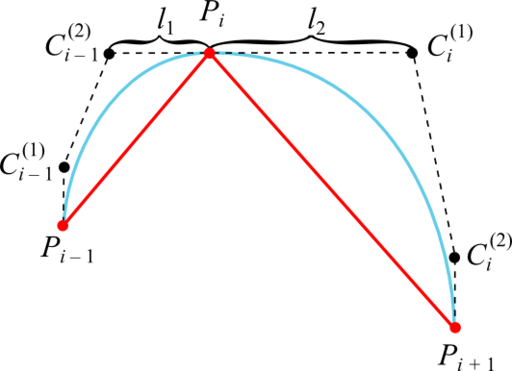
A sufficient condition for attaining defect 2 is that the intermediate control points of the cubic Bezier curve adjacent to a given point of the interpolated sequence lie with this point on one straight line and at the same distance:

As straight lines on which the points C i - 1 (2) , P i and C i (1) lie, it is advisable to take the tangents to the graph of the interpolated function at the points P i . This guarantees the absence of false extremes, since the Bezier curve turns out to be a bounded broken line built on its control points (if this broken line has no self-intersections).
The trial and error method of heuristics for calculating the distance from the point of the interpolated sequence to the intermediate control one turned out to be as follows:
The first and last intermediate control points are equal to the first and last points of the graph, respectively (points C 1 (1) and C n - 1 (2) coincide with points P 1 and P n, respectively).
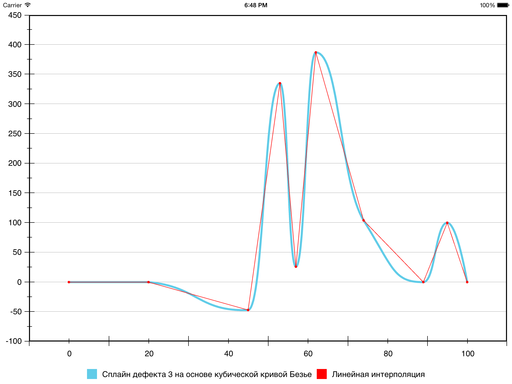
In this case, the result is such a curve:

As you can see, there are no false extremes anymore. However, when compared with linear interpolation, in some places the error is very large. You can make it even less, but even more clever heuristics will be used in the course.
We have come to the current version, reducing the smoothness by one order of magnitude. You can do it again: let the spline have a defect of 3. In fact, the function will not formally be smooth at all: even the first derivative can tolerate discontinuities. But if you tear it gently, visually nothing terrible will happen.
We refuse the requirement of equality of distances from point P i to points C i - 1 (2) and C i (1) , but at the same time we keep them all lying on one straight line:
The heuristics for calculating distances will be:
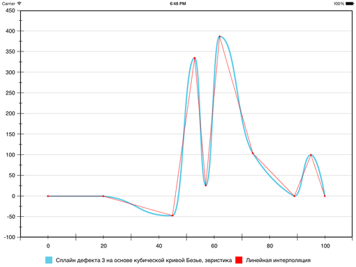
The result is:
As a result, in the sixth segment, the error decreased, and in the seventh segment it increased: Bezier’s curvature turned out to be greater than desired. The situation can be rectified by forcibly reducing the curvature and thereby “pressing” Bezier closer to the line segment that connects the boundary points of the segment. To do this, use the following heuristics:
The result is as follows:
At this decision was made to recognize the goal achieved.
Maybe someone handy code .
Promised review. Of course, before the solution of the problem, we looked at who could boast something, and only then began to figure out how to do it ourselves and, if possible, better. But as soon as they did, it was not without pleasure that we once again walked through the available instruments and compared their results with the results of our experiments. So let's go.

This is very similar to the spline 1 defect discussed above, based on Bezier curves. True, unlike him in its pure form, there are only two false extremes - the first and second segments (we had four). Apparently, some heuristics are added here to the classical search for intermediate control points. But they didn’t save them from all the false extremes.
In the settings, this is called a cubic spline. Obviously, it is also based on Bezier, and here is an exact copy of our result: all four false extrema are in place.
There is another type of interpolation that we did not consider here: B-spline. But for our task, it is clearly not suitable, since it gives this result :)


Here there is a “tangent method” in the variant of equality of distances from the point of the interpolated sequence to the intermediate control ones. There are no false extremums, but there is a relatively large error regarding linear interpolation (the seventh segment).

The picture is very similar to Excel, the same two false extremes in the same places.

There are false extremes and it is clear that the spline of defect 1 based on Bezier is used.
The library is open, so you can look into the code and see this.

Most similar to the Bezier curve of degree n - 1, although in the library itself the graph is called “cubic line”. Strange! Be that as it may, not only are there false extremes, but in principle the interpolation conditions are not fulfilled.
Ultimately, it turns out that Highcharts solved the problem best of the “big guys”. But the method described in this article provides an even smaller error regarding linear interpolation.
In general, we had to do this at the request of buyers, who reported to us "sharp corners" as a bug in our chart engine . We will be glad if the described experience is useful to someone.
Little materiel
Recovery of intermediate values of a function, which in this case is given in tabular form as points P 1 ... P n , is called interpolation. There are many interpolation methods, but all of them can be reduced to finding the n - 1 function to calculate intermediate points on the corresponding segments. In this case, the given points must be computable through the corresponding functions. Based on this, a graph can be built:
The functions f i can be very different, but most often they use polynomials of some degree. In this case, the final interpolating function (piecewise defined on the intervals bounded by points P i ) is called a spline .
')
In different graphing tools — editors and libraries — the problem of “beautiful interpolation” is solved differently. At the end of the article there will be a small overview of the existing options. Why at the end? So that after a number of the above calculations and reflections it was possible to guess which of the "serious guys" use what methods.
Set up experiments
The simplest example is linear interpolation, in which polynomials of the first degree are used, and as a result we get a polyline connecting the given points.
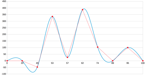
Let's add some specifics. Here is a set of points (taken almost from the ceiling):
0 0 20 0 45 -47 53 335 57 26 62 387 74 104 89 0 95 100 100 0 The result of linear interpolation of these points is as follows:
However, as noted above, sometimes you want to end up with a smooth curve.
What is smoothness? Household answer: no sharp corners. Mathematical: continuity of derivatives. Moreover, in mathematics, smoothness has an order equal to the number of the last continuous derivative, and the area on which this continuity is preserved. That is, if the function has a smoothness of order 1 on the segment [ a ; b ], this means that on [ a ; b ] it has a continuous first derivative, but the second derivative already suffers a gap at some points.
A spline in the context of smoothness is the concept of a defect. A spline defect is the difference between its degree and its smoothness. The degree of the spline is the maximum degree of the polynomials used in it.
It is important to note that the “dangerous” points of the spline (at which smoothness can be broken) are just P i , that is, the junction points of the segments at which the transition from one polynomial to another occurs. All other points are “safe”, because a polynom on the domain of its definition has no problems with the continuity of derivatives.
In order to achieve smooth interpolation, it is necessary to increase the degree of polynomials and choose their coefficients so that the continuity of the derivatives is preserved at the boundary points.
Traditionally, to solve this problem, polynomials of the third degree are used and the continuity of the first and second derivatives is achieved. What turns out is called the cubic spline of defect 1 . Here is how it looks for our data:
The curve is really smooth. But if we assume that this is a schedule of some process or phenomenon that needs to be shown to an interested person, then this method is most likely not suitable. The problem is in false extremes. They appeared due to too much curvature, which was intended to ensure the smoothness of the interpolation function. But this behavior is not at all useful to the viewer, because he is deceived about the peak values of the function. And for the sake of visual visualization of these values, in fact, everything was started.
So you need to look for other solutions.
Another traditional solution, except for cubic splines of defect 1, is Lagrange polynomials. These are polynomials of degree n - 1 that take given values at given points. That is, division into segments does not occur here; the entire sequence is described by one polynomial.
But what happens is:
Smoothness, of course, is present, but visibility has suffered so much that ... perhaps I should look for other methods. On some data sets, the result is normal, but in general, the error with respect to linear interpolation (and, accordingly, false extremes) may be too large - due to the fact that there is only one polynomial for all segments.
In computer graphics, Bezier curves , represented by kth- degree polynomials, are very widely used.
They are not interpolating, because of the k + 1 points involved in the construction, the final curve passes only through the first and the last. The remaining k - 1 points play the role of a kind of "gravitational centers" that attract the curve to itself.
Here is an example of a cubic Bezier curve:
How can this be used for interpolation? On the basis of these curves, it is also possible to construct a spline. That is, each segment of the spline will have its k -th Bezier curve (by the way, k = 1 gives linear interpolation). And the only question is what k to take and how to find k - 1 intermediate point.
There are infinitely many options (since k is not limited by anything), but we will consider the classic: k = 3.
In order for the final curve to be smooth, you need to achieve defect 1 for the spline being made, that is, to preserve the continuity of the first and second derivatives at the junction points of the segments ( P i ), as is done in the classical version of the cubic spline.
The solution to this problem in detail (with source code) is discussed here .
This is what happens on our test suite:
It has become better: there are still false extremes, but at least they are not so different from the real ones.
We think and experiment
You can try to weaken the smoothness condition: require defect 2, not 1, that is, to maintain the continuity of the first derivative alone.
A sufficient condition for attaining defect 2 is that the intermediate control points of the cubic Bezier curve adjacent to a given point of the interpolated sequence lie with this point on one straight line and at the same distance:
As straight lines on which the points C i - 1 (2) , P i and C i (1) lie, it is advisable to take the tangents to the graph of the interpolated function at the points P i . This guarantees the absence of false extremes, since the Bezier curve turns out to be a bounded broken line built on its control points (if this broken line has no self-intersections).
The trial and error method of heuristics for calculating the distance from the point of the interpolated sequence to the intermediate control one turned out to be as follows:
Heuristics 1
The first and last intermediate control points are equal to the first and last points of the graph, respectively (points C 1 (1) and C n - 1 (2) coincide with points P 1 and P n, respectively).
In this case, the result is such a curve:
As you can see, there are no false extremes anymore. However, when compared with linear interpolation, in some places the error is very large. You can make it even less, but even more clever heuristics will be used in the course.
We have come to the current version, reducing the smoothness by one order of magnitude. You can do it again: let the spline have a defect of 3. In fact, the function will not formally be smooth at all: even the first derivative can tolerate discontinuities. But if you tear it gently, visually nothing terrible will happen.
We refuse the requirement of equality of distances from point P i to points C i - 1 (2) and C i (1) , but at the same time we keep them all lying on one straight line:
The heuristics for calculating distances will be:
Heuristics 2
The calculation of l 1 and l 2 is the same as in “heuristics 1”.
At the same time, however, it is worth checking whether the points P i and P i + 1 did not coincide on the ordinate, and, if they did, assume l 1 = l 2 = 0. This will protect the chart from “swelling” on flat segments (which also It is important from the point of view of truthful data display).
At the same time, however, it is worth checking whether the points P i and P i + 1 did not coincide on the ordinate, and, if they did, assume l 1 = l 2 = 0. This will protect the chart from “swelling” on flat segments (which also It is important from the point of view of truthful data display).
The result is:
As a result, in the sixth segment, the error decreased, and in the seventh segment it increased: Bezier’s curvature turned out to be greater than desired. The situation can be rectified by forcibly reducing the curvature and thereby “pressing” Bezier closer to the line segment that connects the boundary points of the segment. To do this, use the following heuristics:
Heuristics 3
If the abscissa of the point of intersection of the tangents at the points P i ( x i , y i ) and P i + 1 ( x i + 1 , y i + 1 ) lies in the segment [ x i ; x i + 1 ], then l 1 or l 2 is set equal to zero. In that case, if the tangent at point P i is directed upwards, we assume zero as the maximum of l 1 and l 2 , if down is the minimum.
The result is as follows:
At this decision was made to recognize the goal achieved.
Maybe someone handy code .
And how do people do something?
Promised review. Of course, before the solution of the problem, we looked at who could boast something, and only then began to figure out how to do it ourselves and, if possible, better. But as soon as they did, it was not without pleasure that we once again walked through the available instruments and compared their results with the results of our experiments. So let's go.
MS Excel
This is very similar to the spline 1 defect discussed above, based on Bezier curves. True, unlike him in its pure form, there are only two false extremes - the first and second segments (we had four). Apparently, some heuristics are added here to the classical search for intermediate control points. But they didn’t save them from all the false extremes.
LibreOffice Calc
In the settings, this is called a cubic spline. Obviously, it is also based on Bezier, and here is an exact copy of our result: all four false extrema are in place.
There is another type of interpolation that we did not consider here: B-spline. But for our task, it is clearly not suitable, since it gives this result :)
Highcharts , one of the most popular JS-libraries for charting
Here there is a “tangent method” in the variant of equality of distances from the point of the interpolated sequence to the intermediate control ones. There are no false extremums, but there is a relatively large error regarding linear interpolation (the seventh segment).
amCharts , another popular JS library
The picture is very similar to Excel, the same two false extremes in the same places.
Coreplot , the most popular graphing library for iOS and OS X
There are false extremes and it is clear that the spline of defect 1 based on Bezier is used.
The library is open, so you can look into the code and see this.
aChartEngine , such as the most popular charting library for Android
Most similar to the Bezier curve of degree n - 1, although in the library itself the graph is called “cubic line”. Strange! Be that as it may, not only are there false extremes, but in principle the interpolation conditions are not fulfilled.
Instead of conclusion
Ultimately, it turns out that Highcharts solved the problem best of the “big guys”. But the method described in this article provides an even smaller error regarding linear interpolation.
In general, we had to do this at the request of buyers, who reported to us "sharp corners" as a bug in our chart engine . We will be glad if the described experience is useful to someone.
Source: https://habr.com/ru/post/264191/
All Articles