Continuously distributed random variables generators
The random number generator is in many ways similar to sex: when it’s good, it’s fine, when it’s bad, it’s still nice (George Marsalya, 1984)
The popularity of stochastic algorithms is growing. Many of them are based on the generation of a large number of different random variables. Not always evenly distributed. Here I tried to collect information about fast and accurate random variable generators with known distributions. Tasks may be different, criteria may be different. The generation time is important to someone, accuracy to someone, cryptostability to someone, speed of convergence to someone. Personally, I proceeded from the assumption that we have a certain basic generator that returns a pseudo-random integer uniformly distributed from 0 to a certain RAND_MAX
unsigned long long BasicRandGenerator() { unsigned long long randomVariable; // some magic here ... return randomVariable; } and that this generator is fast enough. I mean, it's cheaper to generate a dozen random numbers, rather than calculate the logarithm or raise one of them to a power. These can be standard generators: std :: rand (), rand in MATLAB, Java.util.Random, etc. But keep in mind that these generators are rarely suitable for serious work. Often they fail various statistical tests. And also, remember that you are completely dependent on them and it is better to use your own generator to have an idea of its work.
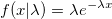
In the article I will talk about algorithms, the essence of which should be clear to anyone who has ever come across the theory of probability. It is not necessary to be familiar with the theory of measure, as a rule, it’s rather enough to understand what the distribution function and the density distribution function are:
')
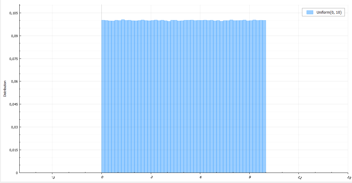
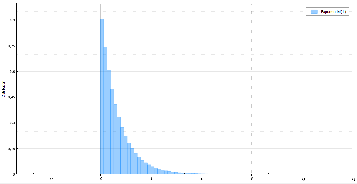
I will accompany each algorithm with a code, a small amount of mathematics and a histogram of ten million generated random variables.
Uniform distribution
Uniform distribution can be used when generating almost any random variable, since there is a very simple and universal method of inversion (inverse transform sampling) : generate a random variable U uniformly distributed from 0 to 1, and return the inverse distribution function (quantile) with the parameter U. Really:

The problem is that the calculation of the inverse distribution function can be long, if analytically possible at all.
With a uniform distribution generator, I hope I don’t need to stop for a long time (with a large number of random variables generated, it’s better to count (b - a) / RAND_MAX only once):
double Uniform(double a, double b) { return a + BasicRandGenerator() * (b - a) / RAND_MAX; } Of course, continuity is just an abstraction. In the real world, and in this case, specifically, this implies a rather small discretization step. It is worth noting an important thing. If you generate a random number evenly distributed from 0 to 1, then 32 bits are not enough to cover all the values that double can take on this range (although, for a float, this is more than enough). For better quality, you must either generate 64-bit integers, or combine two 32-bit integers.
Normal distribution
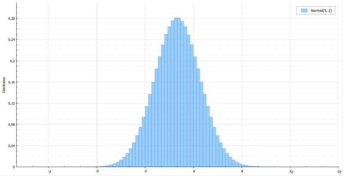
The inversion method will require the calculation of the inverse error function. If you do not use special approximating functions, it is difficult and incredibly long. For a normal quantity, there is the Box-Muller method. It is quite simple and widespread. Its obvious disadvantage is the computation of transcendental functions. On Habré, the polar method has already been mentioned, which helps to avoid counting sine and cosine. But we still have to read the logarithm and the root of it. The beautifully named Ziggurat method, invented by George Marsalla, the author of the same polar method, works much faster.
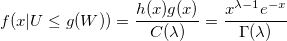
The polar method is an example of a sample with a deviation (acceptance-rejection sampling) . Literally, you generate a value and accept it if it fits; otherwise, reject and generate it again. The main example: you need to generate a random variable with a density f (x), but it is too difficult to do with a simple inversion method. On the other hand, you can generate a random variable with a density g (x) not very different from f (x). In this case, you take the smallest constant M, such that M> 1 and almost everywhere f (x) <Mg (x), and perform the following algorithm:
- We generate a random variable X from the distribution g (x) and a random variable U, uniformly distributed from 0 to 1.
- If U <f (X) / Mg (X) - return X, otherwise - repeat again.
The probability of accepting a random variable:

The less you choose M - the more this probability - the faster the generator will work.
Proof of the algorithm:
Taking advantage of the fact that the probability of the origin of two events A and B is equal to

Let us calculate the probability of accepting a random variable X with the distribution density function g (x) and the distribution function G (x), but under the condition that it is less than a certain given parameter x:

And then according to the Bayes theorem:

Let us calculate the probability of accepting a random variable X with the distribution density function g (x) and the distribution function G (x), but under the condition that it is less than a certain given parameter x:
And then according to the Bayes theorem:
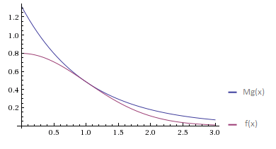
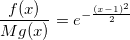
For example, we generate a module of a standard normal value. By virtue of the symmetry of the normal distribution, the resulting value can be multiplied by a random variable taking values of +1 and -1 with equal probabilities, and thus a standard normally distributed quantity X. Any normal quantity is obtained from the standard multiplication by sigma and a shift by mu. Density distribution function | X |:

We will try to approximate it with the density function of the standard exponential distribution. I am running a little ahead, because I have not yet spoken about the exponential distribution. It is generated simply by the notorious inversion method - we take the value U uniformly distributed on [0, 1] and return -ln (U).

The minimum value of M, satisfying the condition f (x) <Mg (x), is achieved at x = 1:

Then:
And the algorithm for generating a normal random variable will be as follows:
- We generate U - uniformly distributed random variable on [0, 1].
- We generate an exponentially distributed random variable E (about an algorithm that is faster than the calculation of -ln (U), I will tell further).
- If U <exp (- (E - 1) 2 ) - then | X | = E, otherwise we return to the first step.
- We generate a new U. If U <0.5, then we return - | X |, or | X | otherwise.
It is easy to see that:

And this means that instead of U, you can generate another exponentially distributed quantity and not consider an exponential function. The new algorithm will look like this:
- We generate standard exponentially distributed random variables E 1 and E 2 .
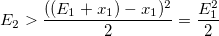
- If E 2 > (E 1 - 1) 2/2, then we take | X | = E 1 , otherwise go back.
- We generate U. If U <0.5, then we return - | X |, or | X | otherwise.
Another point: if the value of E 1 is accepted, the difference E 2 - (E 1 - 1) 2/2 will also be distributed exponentially and independently of E 1 . Therefore, it can be memorized and used next time instead of E 1 .
Evidence
The exponential distribution has the absence of memory property:

This means that the difference distribution function:

This means that the difference distribution function:
The general problem of a sample with a deviation is the selection of such a random variable with a distribution density g (x) so that the deviations are as small as possible. To solve this problem, there are many extensions. The method itself is the basis for almost all subsequent algorithms, including Ziggurat. The essence of the latter is the same: we try to cover the density function of the normal distribution with a similar and simpler function and return the values that fall under the curve. The function is unique and resembles a multistage structure, from which, in fact, this is the name of the algorithm.
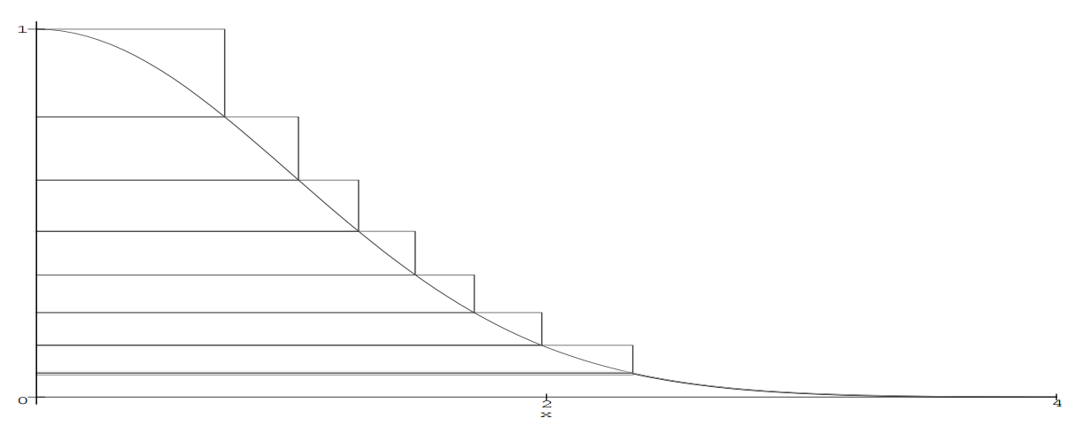
Ziggurat is constructed as follows. At the foot of the function f (x), the points x 1 and y 0 = f (x 1 ) are selected. The area under the rectangle from (0,0) to (x 1 , y 0 ) + the area under the tail of the function f (x> x 1 ) = A. So we built the base layer. Another rectangle is placed on top of it, such that its width is x 1 , and the height is y 1 = A / y 0 and thus its area will be A. This rectangle already includes points that lie above the function f (x), for example (x 1 , y 1 ). The second rectangle intersects the function f (x) at the point (x 2 , y 1 ) - this will be the coordinate of the lower right point of the third rectangle, which is superimposed in the same way as the second, so that its area is A. This continues until we will not build a ziggurat to the top of the function. The area of each step will be equal to A. Further algorithm (without processing to fall into the base layer) :
- Randomly and uniformly select the rectangle i and generate a uniformly distributed value X from 0 to x i
- If X <x i + 1 , then we definitely got under the curve - return X.
- We generate a new uniformly distributed quantity Y from y i to y i + 1 . If the point with coordinates (X, Y) lies under the curve, that is, Y <f (X) - we return X. Otherwise we return to the first step.
What to do if you hit the base layer? You can also make a rectangle from it with area A by entering an imaginary point x 0 = A / y 0 . Then the area of the rectangle from (0,0) to (x 0 , y 0 ) will also be equal to A. The difference in the base layer is that if we do not fall under the curve in the new imaginary rectangle, then we should not reject x - we just hit the tail. For the tail, George Marsalla suggests using the same method that we had previously considered - a sample with a deviation. Only with some changes:
- We generate standard exponentially distributed random variables E 1 with density x 1 and E 2 with unit density.
- If E 2 > E 1 2/2, then we take | X | = E 1 + x 1 , otherwise we go back.
- We generate U. If U <0.5, then we return - | X |, or | X | otherwise.
Proof for tail
We know that the random variable | X | > x 1 . We will try to construct for it a sampling algorithm with a deviation using E 1 + x 1 , where E 1 is an exponentially distributed random variable with density x 1 . Density distribution function E 1 + x 1 :

To know the value of M, we need to find the maximum of the ratio of functions:

The point x corresponding to the maximum fraction will deliver the maximum degree of the exponent. Equating the derivative of degree to zero, we find the corresponding x:

We get the boundary for a uniform random variable:

And then the condition for accepting a random variable will be:
To know the value of M, we need to find the maximum of the ratio of functions:
The point x corresponding to the maximum fraction will deliver the maximum degree of the exponent. Equating the derivative of degree to zero, we find the corresponding x:
We get the boundary for a uniform random variable:
And then the condition for accepting a random variable will be:
Then the algorithm will look completely like this:
- Randomly and uniformly select the rectangle i and generate a uniformly distributed value X from 0 to x i .
- If X <x i + 1 , then we definitely got under the curve - return X.
- If you hit the base layer, that is, i = 0, then we run the algorithm for the tail and return its result.
- We generate a new uniformly distributed quantity Y from y I to y i + 1 . If the point with coordinates (X, Y) lies under the curve, that is, Y <f (X) - we return X. Otherwise we return to the first step.
The question is how to find the constants A and x 1 depending on the number of rectangles? You can find them by an ordinary numerical method. We take the initial assumption x 1 , build the base layer, calculate A and build the ziggurat until we have built the required number of rectangles. If we were above the function, it means we took too small a value of x 1 and a too large value of A - try to build with new values again.
The algorithm itself can be accelerated by various tricks of work with 32-bit integers, removing unnecessary multiplication. For more information, see George Marsaglia and Wai Wan Tsang, "The Ziggurat Method for Generating Random Variables." Here I imagine not fully optimized, but clear code (given that we can generate exponential distribution).
static double stairWidth[257], stairHeight[256]; const double x1 = 3.6541528853610088; const double A = 4.92867323399e-3; /// area under rectangle void setupNormalTables() { // coordinates of the implicit rectangle in base layer stairHeight[0] = exp(-.5 * x1 * x1); stairWidth[0] = A / stairHeight[0]; // implicit value for the top layer stairWidth[256] = 0; for (unsigned i = 1; i <= 255; ++i) { // such x_i that f(x_i) = y_{i-1} stairWidth[i] = sqrt(-2 * log(stairHeight[i - 1])); stairHeight[i] = stairHeight[i - 1] + A / stairWidth[i]; } } double NormalZiggurat() { int iter = 0; do { unsigned long long B = BasicRandGenerator(); int stairId = B & 255; double x = Uniform(0, stairWidth[stairId]); // get horizontal coordinate if (x < stairWidth[stairId + 1]) return ((signed)B > 0) ? x : -x; if (stairId == 0) // handle the base layer { static double z = -1; double y; if (z > 0) // we don't have to generate another exponential variable as we already have one { x = Exponential(x1); z -= 0.5 * x * x; } if (z <= 0) // if previous generation wasn't successful { do { x = Exponential(x1); y = Exponential(1); z = y - 0.5 * x * x; // we storage this value as after acceptance it becomes exponentially distributed } while (z <= 0); } x += x1; return ((signed)B > 0) ? x : -x; } // handle the wedges of other stairs if (Uniform(stairHeight[stairId - 1], stairHeight[stairId]) < exp(-.5 * x * x)) return ((signed)B > 0) ? x : -x; } while (++iter <= 1e9); /// one billion should be enough return NAN; /// fail due to some error } double Normal(double mu, double sigma) { return mu + NormalZiggurat() * sigma; } Exponential distribution
It has already been said that for an exponential distribution one can take the logarithm of a uniformly distributed quantity and what can be done to generate faster. Since any exponential value is obtained from the standard division by density, the generation can be made notorious Ziggurat. In the case of hitting the tail, you can run the algorithm on the new and add to the resulting value x 1 :
Evidence
It is necessary to prove that for E> x 1 the distribution function E - x 1 will also be distributed exponentially. This is possible due to the previously mentioned lack of memory in the exponential distribution:

A couple more facts: if you use a table with 255 rectangles, then the probability of accepting from the first time for the exponential distribution is 0.989, for a normal one - 0.993. In MATLAB version 5, Ziggurat is used for normal distribution (the polar method was used before). In R, for normal values, as far as I know, the inverse error function is approximated by polynomials and the inversion method is used.
static double stairWidth[257], stairHeight[256]; const double x1 = 7.69711747013104972; const double A = 3.9496598225815571993e-3; /// area under rectangle void setupExpTables() { // coordinates of the implicit rectangle in base layer stairHeight[0] = exp(-x1); stairWidth[0] = A / stairHeight[0]; // implicit value for the top layer stairWidth[256] = 0; for (unsigned i = 1; i <= 255; ++i) { // such x_i that f(x_i) = y_{i-1} stairWidth[i] = -log(stairHeight[i - 1]); stairHeight[i] = stairHeight[i - 1] + A / stairWidth[i]; } } double ExpZiggurat() { int iter = 0; do { int stairId = BasicRandGenerator() & 255; double x = Uniform(0, stairWidth[stairId]); // get horizontal coordinate if (x < stairWidth[stairId + 1]) /// if we are under the upper stair - accept return x; if (stairId == 0) // if we catch the tail return x1 + ExpZiggurat(); if (Uniform(stairHeight[stairId - 1], stairHeight[stairId]) < exp(-x)) // if we are under the curve - accept return x; // rejection - go back } while (++iter <= 1e9); // one billion should be enough to be sure there is a bug return NAN; // fail due to some error } double Exponential(double rate) { return ExpZiggurat() / rate; } Gamma distribution


Algorithms for generating here are more complicated, so I will not describe their evidence here, I give only examples. To generate a standard value (theta = 1), four algorithms are used, each depending on k.
- If k or 2k is an integer and k <5 is a GA algorithm.
- If k <1 - GS algorithm.
- If 1 <k <3 - GF algorithm.
- If k> 3 - GO algorithm.
Non-standard random variable with gamma distribution, obtained from the standard multiplication by theta.
GA algorithm
If we add two random variables with the gamma distribution with the parameters k1 and k2, we get a random variable with the gamma distribution and with the parameter k1 + k2. Another property - if theta = k = 1, then it is easy to verify that the distribution will be exponential. Therefore, if k is integer - then you can simply sum up k random variables with standard exponential distribution.
double GA1(int k) { double x = 0; for (int i = 0; i < k; ++i) x += Exponential(1); return x; } If k is not integer, but 2k is integer, then instead of one of the exponential random variables in total, one can use half of the square of the normal value. Why is it possible, it will become clear later.
double GA2(double k) { double x = Normal(0, 1); x *= 0.5 * x; for (int i = 1; i < k; ++i) x += Exponential(1); return x; } GS Algorithm
- We generate the standard exponentially distributed quantity E and the quantity U, uniformly distributed from 0 to 1 + k / e. If U <= 1, then go to step 2. Otherwise, to step 3.
- Set x = U 1 / k . If x <= E, then return x, otherwise go back to step 1.
- Set x = -ln ((1 - U) / k + 1 / e). If (1 - k) * ln (x) <= E, then we return x, otherwise we return to step 1.
double GS(double k) { // Assume that k < 1 double x = 0; int iter = 0; do { // M_E is base of natural logarithm double U = Uniform(0, 1 + k / M_E) double W = Exponential(1) if (U <= 1) { x = pow(U, 1.0 / k); if (x <= W) return x; } else { x = -log((1 - U) / k + 1.0 / M_E); if ((1 - k) * log(x) <= W) return x; } } while (++iter < 1e9); // excessive maximum number of rejections return NAN; // shouldn't end up here } GF algorithm
As far as I know, the author of this algorithm, a professor at the University of North Carolina, J. S. Fishman, did not publish his achievement. The algorithm itself works for k> 1, however, its average execution time increases proportionally to sqrt (k), therefore it is effective only for k <3. Algorithm:
- We generate two independent random variables E 1 and E 2 with standard exponential distribution.
- If E 2 <(k - 1) * (E 1 - ln (E 1 ) - 1), then go back to step 1.
- Return x = k * E 1
Evidence
Theorem. Let U be a uniformly distributed random variable on [0, 1] and W is an exponentially distributed random variable with a density of 1 / lambda. Let be:

If g (W)> = U, then W has a gamma distribution with the lambda parameter:

Evidence. Distribution density function W:

In this way,

Since U has a uniform distribution,

if 0 <g (x) <1. Then the unconditional probability:

As a result, the conditional probability density:
qed
The generator efficiency is determined by the probability that U <= g (W), which is equal to C (lambda). For large values of the \ lambda parameter, using the Stirling approximation, we can roughly calculate the probability:

The algorithm becomes inefficient with a growing lambda.
If g (W)> = U, then W has a gamma distribution with the lambda parameter:
Evidence. Distribution density function W:
In this way,
Since U has a uniform distribution,
if 0 <g (x) <1. Then the unconditional probability:
As a result, the conditional probability density:
qed
The generator efficiency is determined by the probability that U <= g (W), which is equal to C (lambda). For large values of the \ lambda parameter, using the Stirling approximation, we can roughly calculate the probability:
The algorithm becomes inefficient with a growing lambda.
double GF(double k) { // Assume that 1 < k < 3 double E1, E2; do { E1 = Exponential(1); E2 = Exponential(1); } while (E2 < (k - 1) * (E1 - log(E1) - 1)); return k * E1; } GO Algorithm
The algorithm of Dieter and Arens is based on the asymptotic normality of the distribution with increasing parameter, and therefore is faster for large k. It works for k> 2.533, but not as efficient as the Fisher algorithm for k <3. First, you need to set some constants (depending only on k).
void setupConstants(double k) { m = k - 1; s_2 = sqrt(8.0 * k / 3) + k; s = sqrt(s_2); d = M_SQRT2 * M_SQRT3 * s_2; b = d + m; w = s_2 / (m - 1); v = (s_2 + s_2) / (m * sqrt(k)); c = b + log(s * d / b) - m - m - 3.7203285; } double GO(double k) { // Assume that k > 3 double x = 0; int iter = 0; do { double U = Uniform(0, 1); if (U <= 0.0095722652) { double E1 = Exponential(1); double E2 = Exponential(1); x = b * (1 + E1 / d); if (m * (x / b - log(x / m)) + c <= E2) return x; } else { double N; do { N = Normal(0, 1); x = s * N + m; // ~ Normal(m, s) } while (x < 0 || x > b); U = Uniform(0, 1); double S = 0.5 * N * N; if (N > 0) { if (U < 1 - w * S) return x; } else if (U < 1 + S * (v * N - w)) return x; if (log(U) < m * log(x / m) + m - x + S) return x; } } while (++iter < 1e9); return NAN; // shouldn't end up here; } As in the case of previous distributions, any value with a gamma distribution is generated from the standard multiplication by the theta parameter. Being able to generate uniform, normal, exponential and gamma distributions, you most likely can easily get most of the other distributions, since they can easily be expressed through the aforementioned ones.
Cauchy distribution


One way to quickly get a random variable with a Cauchy distribution is to take two normal random variables and divide them into each other. Is it faster? You can use the usual method of inversion, but it will require the calculation of tangent. This is even slower.

Or not?
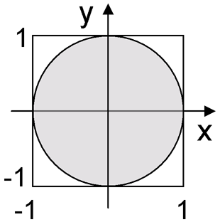
Remember the polar method of George Marsaly? - . . x y [-1, 1]x[-1, 1]. (0, 0) — x/y, — x y . , , 0.01.
double Cauchy(double x0, double gamma) { double x, y; do { x = Uniform(-1,1); y = Uniform(-1,1); } while (x * x + y * y > 1.0 || y == 0.0); return x0 + gamma * x / y; } 
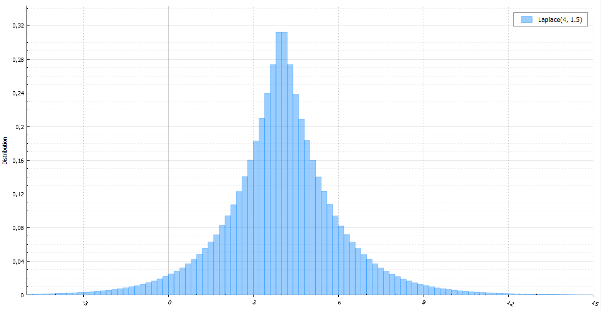
— , .
double Laplace(double mu, double b) { double E = Exponential(1.0 / b); return mu + (((signed)BasicRandGenerator() > 0) ? E : -E); } 

, , :
double Levy(double mu, double c) { double N = Normal(0, 1); return mu + c / (N * N); } -

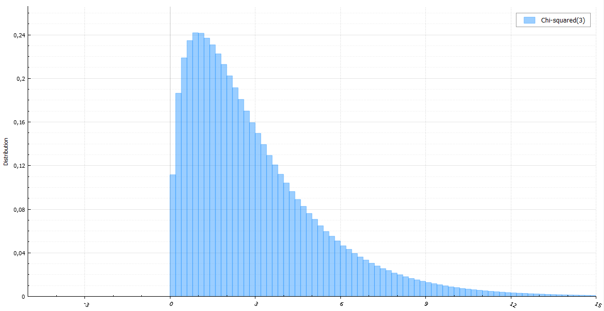
, - k — k . , k k/2 ( ). GA2:
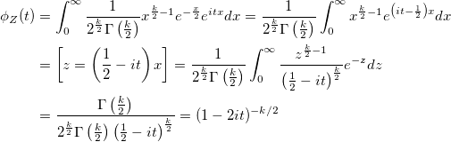
Evidence
, — :

:

E — :

:

:

-, :
. , :

, :

qed
:
E — :
:
:
-, :
. , :
, :
qed
double ChiSquared(int k) { // ~ Gamma(k / 2, 2) if (k >= 10) // too big parameter return GO(0.5 * k); double x = ((k & 1) ? GA2(0.5 * k) : GA1(k >> 1)); return x + x; } : (x, y), (0,0) .


, , . , -, - — . , , , , / -. , . :
double LogNormal(double mu, double sigma) { return exp(Normal(mu, sigma)); } 
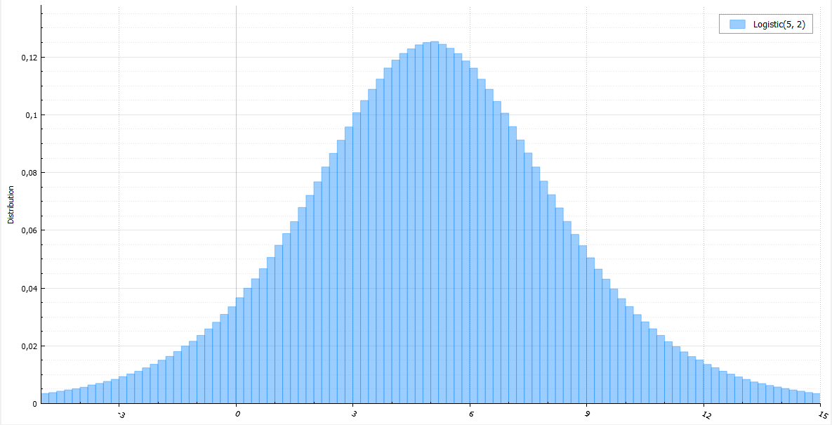
, , :
double Logistic(double mu, double s) { return mu + s * log(1.0 / Uniform(0, 1) - 1); } , :
double Erlang(int k, double l) { return GA1(k) / l; } double Weibull(double l, double k) { return l * pow(Exponential(1), 1.0 / k); } double Rayleigh(double sigma) { return sigma * sqrt(Exponential(0.5)); } double Pareto(double xm, double alpha) { return xm / pow(Uniform(0, 1), 1.0 / alpha); } double StudentT(int v) { if (v == 1) return Cauchy(0, 1); return Normal(0, 1) / sqrt(ChiSquared(v) / v); } double FisherSnedecor(int d1, int d2) { double numerator = d2 * ChiSquared(d1); double denominator = d1 * ChiSquared(d2); return numerator / denominator; } double Beta(double a, double b) { double x = Gamma(a); return x / (x + Gamma(b)); } Implementing these and other C ++ generators 17
Source: https://habr.com/ru/post/263993/
All Articles