Content

1. What is a tensor and what is it for?
2. Vector and tensor operations. Ranks of tensors
3. Curved coordinates
4. Dynamics of a point in the tensor representation
5. Actions on tensors and some other theoretical questions
6. Kinematics of free solid. Nature of angular velocity
7. The final turn of a solid. Rotation tensor properties and method for calculating it
8. On convolutions of the Levi-Civita tensor
9. Conclusion of the angular velocity tensor through the parameters of the final rotation. Apply head and maxima
10. Get the angular velocity vector. We work on the shortcomings
11. Acceleration of the point of the body with free movement. Solid Corner Acceleration
12. Rodrig – Hamilton parameters in solid kinematics
13. SKA Maxima in problems of transformation of tensor expressions. Angular velocity and acceleration in the parameters of Rodrig-Hamilton
14. Non-standard introduction to solid body dynamics
15. Non-free rigid motion
16. Properties of the inertia tensor of a solid
17. Sketch of nut Janibekov
18. Mathematical modeling of the Janibekov effect

Introduction

Last time we considered one of the ways to obtain differential equations of motion of a rigid body based on the d'Alembert principle. We settled on the general form of the equations of motion.


However, carefully looking at these equations, I should criticize - the fact is that the number of unknowns in these equations is too large. The unknowns include pole acceleration. and angular acceleration of the body , and also reactions of communications . And if the body movement is limited by at least one bond, the number of unknown quantities in (1) and (2) exceeds the number of equations.
')
This is because the left side of equations (1) and (2) contains accelerations calculated for the case of free body motion, that is, they have redundant coordinates. Therefore, system (1), (2) should be supplemented with equations of bonds describing the constraints imposed by the constraints on the coordinates, velocities and accelerations of points of the body.

This is what we are going to do now - let's see what equations (1) and (2) turn into when adding link equations, and what the resulting equations give us in a practical sense.

1. Equations of motion of a free solid

A free body is a body whose movement is not limited to bonds. Accordingly, in the equations (1) and (2) the extra unknowns disappear and they turn into


And for a free body it makes no sense to use an arbitrary pole - it is better to change the center of reduction of the inertial force systems to the center of mass of the body, writing down the equations of motion in a simpler form


Equations (5) and (6) are the differential equations of free motion of a rigid body. They can be resolved with respect to accelerations and integrated numerically, given the initial conditions.

2. Equations of motion of a rigid body with one fixed point

Now suppose that the movement of the body is limited by a spherical hinge located at the point . Then, by choosing a pole at this fixed point, we can add a coupling equation




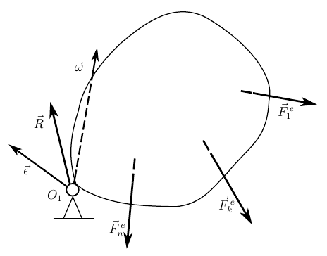
The reaction of the spherical hinge, is expressed by one force therefore, taking into account (7), equations (1) and (2) can be rewritten as


where as strength attached at the point so we finally get


Equation (8) allows us to determine the angular acceleration of the body, based on the initial conditions of the problem and the known active forces applied to the body, and equation (9) makes it possible, knowing the angular acceleration, to find the reaction of the spherical hinge. Thus, we obtain the differential equations of spherical motion.

3. Rotational movement of the body. The moment of inertia of the body relative to the axis

Rotational motion is called the movement of a body when its two points remain motionless at any moment in time. If we express this fact with the help of equations, then we can write the following equations of relations




Condition (10) expresses the immobility of one of the points of the body, and condition (11) - the invariance of the direction of the axis of rotation of the body. Based on (11), one can write out the angular velocity and angular acceleration of the body through the parameters of the final turn


Substituting (12) and (10) into equation (2)


Considering that we have two connections, and accordingly two reactions from bearings, on which the body rotates. And you can immediately take into account that , since the first reaction is applied at the point . In addition, we perform the scalar multiplication of the last equation by the orth of the axis of rotation


Consider that the moment of the second reaction can be calculated as , wherein that is, we get


The second components in both parts of this equation are mixed products of coplanar vectors and are zero, as a result, we have


- differential equation of rotation of the body around a fixed axis, where


called the moment of inertia of a solid relative to the axis of rotation , and


- the projection of the vector moment relative to a fixed point on the axis passing through this point or - the moment of force relative to the axis .

Expression (14) is extremely interesting. If we rewrite it in tensor form, then we get the formula


allowing, using the well-known inertia tensor of a solid body, to determine its moment of inertia about the axis of rotation of interest to us, whose direction in space is given by an ort . The moment of inertia (16) is a scalar quantity characterizing the distribution of body mass around the axis of rotation. This value, as well as equation (13), is well known from the general course of theoretical mechanics.

4. Translational body movement

In the progressive movement, the bonds imposed on the body prevent its rotation. In this case, we can write obvious equalities.


Assuming the ideality of relationships, we can write down the condition imposed on their reactions


Where - vector tangent to the trajectories of points of the body. In the case of translational motion, the trajectories of all its points are the same, and hence the vector of the tangent to the trajectory is the same for all points. Taking into account (17) and (18), we can rewrite equation (1)


or


- the differential equation of the translational motion of the body in projections on the tangent to the trajectories of its points.

Conclusion

In this article, we examined how the general equations of motion of a rigid body (1) and (2) are transformed if we supplement them with equations of constraints. At the same time, we easily and naturally constructed differential equations of motion for all special cases of body motion, studied by theoretical mechanics.

Thanks

In preparing this article , the method proposed by the SeptiM user was used . In connection with the obvious convenience of work, I want to express my gratitude to the author for the work he has done.

To be continued...