Automatic textual key detection (Sentiment Analysis)
For a short time of my learning process, I realized one thing - knowledge needs to be shared. I realized this a long time ago, but laziness to overcome and find time does not always work.
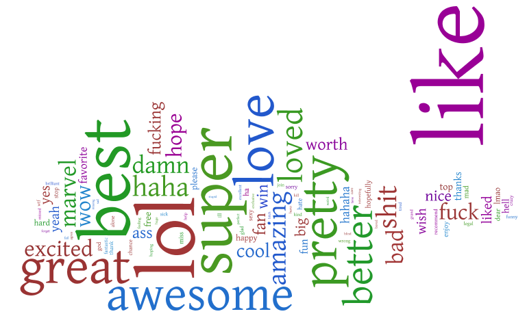
This article will discuss the use of various machine learning methods to solve problems associated with the processing of natural language (NLP). One of these problems is the automatic determination of the emotional color (positive, negative, neutral) of textual data, that is, sentiment analysis. The purpose of this task is to determine whether the given text (say, a film review or commentary) is positive, negative or neutral in its effect on the reputation of a particular object. The difficulty of analyzing the tonality lies in the presence of an emotionally enriched language - slang, polysemy, uncertainty, sarcasm, all these factors mislead not only people, but also computers.
')
On Habré more than once appeared articles related to the definition of tonality 1 , 2 , 3 . Anyway, this topic is one of the most discussed around the world recently [1, 2, 3, 4].
Immediately I will discuss that you will not find any particular innovations in this article, this material can most likely serve as a tutorial for newcomers in the field of machine learning and NLP, which I am. The main material that I used you can find on this link . The entire source code can be found at this link .
So, what is the problem and how to solve it?
Suppose we have a text message (film description, review, comments):
“This film made me upset. It’s just that you’ve taken your time.
Or:
“The best movie I've ever seen !!! Musical composition, actors, scenario, etc. all this stuff are just amazing !!! ”
In the first example, the system should produce a negative result, since the comment is negative, and in the second, respectively, positive. Such tasks in machine learning are called classification, and the method is learning with a teacher. That is, at first, the algorithm on the training sample is “trained”, preserving the necessary coefficients and other data of the model, then, upon entering new data, with a certain probability classifies them. By coefficient, I mean something like this:

Where beta values are our coefficients derived from learning from test data. As we see, this formula ultimately returns a value from 0 to 1 (see sigmoid for more details), that is, the closer to 0, the greater the likelihood that the text carries negative information.
For the training sample, we used an open dataset from www.kaggle.com , namely, a dataset that includes data from 50,000 IMDB movie reviews, specially selected for tonality analysis. The tonality metric is a binary value, that is, IMDB rating <5 is awarded a value of 0, and rating> = 7 is awarded a value of 1.
Each record of this dataset consists of the following fields:
So, we proceed directly to solving the problem. The entire algorithm described in this article is implemented in python (v. 2.7). For readability, I have broken the algorithm into the following steps:
Pre-processing is required before any data processing. In this stage, all html tags, punctuation, symbols are removed. This operation is performed using the python library - “Beautiful Soup”. Also, all numbers and links in the text are replaced by tags,. Further in the text there are so-called “stop words” - these are frequent words in a language that basically do not carry any semantic meaning (for example, in English these are words like “the, at, about ...”). Stop words are removed using the Python Natural Language Toolkit (NLTK) package. After preprocessing the source text, we get the following:
[biography, part, feature, film, remember, going, see, cinema, originally] - That is, a set of words.
At this stage, it is possible to further refine further by modifying each word to its initial form (stemming), etc. But for this experiment, I decided to limit myself to this.
The fact is that the computer, as well as mathematical formulas, is easier to work with numbers, and not a set of words. Therefore, we need to present any text as a vector of numbers. To do this, you can create a dictionary with all the words, i.e. combine all the words found in the texts into one large dictionary, or use ready-made dictionaries (Dahl or Zaliznyak), and replace the words from the text with an index in the dictionary. That is, suppose we have only three reviews with the following pre-processed word vectors:
Combining all the words from the list into one we get the following sorted dictionary (let's call it as a basis vector):
[biography, cinema, feature, film, going, originally, part, remember, see]
Replacing the previous vectors with the index of the word in the dictionary, we get the following:
Having done this work for all reviews, we can get a fairly large list (in my example, I took 5,000 of the most common words). These vectors are called “property vectors” or “features vector”. In this way, we get vectors for each test recall, then we can compare these vectors using standard metrics such as Euclidean distance, cosine distance, etc. This approach is called “bag of words” or “Bag-Of-Words”.
The first approach is a fairly common method and is quite simple to implement, but it is not excluded from the shortcomings. When comparing two vectors, an exact match of words is used, and we lose important information. One of these "missing" information is the semantics of the word. For example, we can easily replace the word “black” with the word “dark”, since their meaning is very similar. Such words can be called - semantic similar words. The group of such words includes synonyms, hyponyms, hyperonyms, etc.
In an alternative approach, we will try to replace each word in the list with the number of its semantic group. As a result, we get something like a "bag of words", but with a deeper meaning. For this, Google’s Word2Vec technology is used. It can be found in the gensim library package, with built-in Word2Vec models.
The essence of the Word2Vec model is as follows: a large amount of text is given at the entrance (in our case approximately 10,000 reviews), at the output we get a weighted vector for each word, a fixed length (the length of the vector is set manually), which is found in dataset. For example, for the word men, comparing with all words and sorting in descending order, I got the following result (I chose the cosine distance for the proximity measure):
Semantic words close to 'man'
You can find out more about how the Word2Vec model works at this link .
Further, clustering is used to combine similar words. Yes, there is another abstruse word - clustering. I will not dwell on this in detail, the article in the wiki ( sigmoid ) I think will explain everything well. But let me tell you the essence of the most primitive clustering algorithm (K-means): suppose we have a certain number of clusters N, the algorithm learning the training data divides them into clusters and finds the centers of each of them, then when entering the test data, the algorithm assigns it a cluster number, center which is the closest to him. In this case, I just took the number of words in the dictionary and divided it into 5, assuming that there would be an average of 5 words in each cluster. On average, I had ~ 3000 clusters. Next, we do the same thing as in the first “Bag-Of-Words” approach, replacing each word with a cluster index, only this time we have something like “Bag-Of-Clusters”. Full source code with explanations on this method, you can get at this link .
So, at the bathing stage, we have already deleted all unnecessary things, transformed the text into a vector, and now we are entering the home straight. The Random Forest Classifications Algorithm is used for document classifications in this experiment. The algorithm is already implemented in the scikit-learn package, all we can do is feed our text data and specify the number of trees. Then the algorithm takes over, trains on the training set, saves all the necessary data.
In short, I launched a classifier based on both approaches for obtaining eigenvectors. Here are some interesting results:
Considering the fact that the launch of Word2Vec took me 2 hours on my old laptop, it showed a relatively better result than the good old Bag-Of-Words.
[1] I. Chetviorkin, P. Braslavskiy, N. Loukachevich, “Sentiment Analysis Track at ROMIP 2011,” In Computational Linguistics and Intellectual Technologies: Proceedings of the International Conference “Dialog 2012”, Bekasovo, 2012, pp. 1-14.
[2] AA Pak, SS Narynov, AS Zharmagambetov, SN Sagyndykova, ZE Kenzhebayeva, I. Turemuratovich, “The method of synonyms extraction from unannotated corpus,” In proc. of DINWC2015, Moscow, 2015, pp. 1-5
[3] T. Mikolov, K. Chen, G. Corrado, J. Dean, “Efficient Estimation of Word Representations in Vector Space,” In Proc. of Workshop at ICLR, 2013.
[4] P. Bo and L. Lee, “A Sentimental Education: Using Subjectivity Analysis”, “In Proceedings of the ACL, 2004”
[5] T. Joachims, “Text categorization with support vector machines: Learning with many relevant features,” In European Conference on Machine Learning (ECML), Springer Berlin / Heidelberg, 1998, pp. 137-142
[6] PD Turney, “Thumbs up or thumbs down? Semantic orientation applied to unsupervised classification of reviews, “40th Annual Meeting of the Association for Computational Linguistics (ACL'02), Philadelphia, Pennsylvania, 2002, pp. 417-424.
[7] A. Go, R. Bhayani, L. Huang, “Twitter Sentiment Classification Using Distant Supervision,” Technical report, Stanford. 2009
[8] J. Furnkranz, T. Mitchell, and E. Riloff, “A Categorization Case on the WWW,” A AAI / ICML Workshop for Learning for Text Categorization, 1998, pp. 5-12.
[9] MF Caropreso, S. Matwin, F. Sebastiani, “PhDorses for automated textual categorization,” “pp. 78-102.
This article will discuss the use of various machine learning methods to solve problems associated with the processing of natural language (NLP). One of these problems is the automatic determination of the emotional color (positive, negative, neutral) of textual data, that is, sentiment analysis. The purpose of this task is to determine whether the given text (say, a film review or commentary) is positive, negative or neutral in its effect on the reputation of a particular object. The difficulty of analyzing the tonality lies in the presence of an emotionally enriched language - slang, polysemy, uncertainty, sarcasm, all these factors mislead not only people, but also computers.
')
On Habré more than once appeared articles related to the definition of tonality 1 , 2 , 3 . Anyway, this topic is one of the most discussed around the world recently [1, 2, 3, 4].
Immediately I will discuss that you will not find any particular innovations in this article, this material can most likely serve as a tutorial for newcomers in the field of machine learning and NLP, which I am. The main material that I used you can find on this link . The entire source code can be found at this link .
So, what is the problem and how to solve it?
Suppose we have a text message (film description, review, comments):
“This film made me upset. It’s just that you’ve taken your time.
Or:
“The best movie I've ever seen !!! Musical composition, actors, scenario, etc. all this stuff are just amazing !!! ”
In the first example, the system should produce a negative result, since the comment is negative, and in the second, respectively, positive. Such tasks in machine learning are called classification, and the method is learning with a teacher. That is, at first, the algorithm on the training sample is “trained”, preserving the necessary coefficients and other data of the model, then, upon entering new data, with a certain probability classifies them. By coefficient, I mean something like this:
Where beta values are our coefficients derived from learning from test data. As we see, this formula ultimately returns a value from 0 to 1 (see sigmoid for more details), that is, the closer to 0, the greater the likelihood that the text carries negative information.
For the training sample, we used an open dataset from www.kaggle.com , namely, a dataset that includes data from 50,000 IMDB movie reviews, specially selected for tonality analysis. The tonality metric is a binary value, that is, IMDB rating <5 is awarded a value of 0, and rating> = 7 is awarded a value of 1.
Each record of this dataset consists of the following fields:
- ID - a unique identifier for each review;
- Sentiment - the tonality of the review; 1 or 0;
- Review - Review text.
Algorithm
So, we proceed directly to solving the problem. The entire algorithm described in this article is implemented in python (v. 2.7). For readability, I have broken the algorithm into the following steps:
Step 1. Pretreatment
Pre-processing is required before any data processing. In this stage, all html tags, punctuation, symbols are removed. This operation is performed using the python library - “Beautiful Soup”. Also, all numbers and links in the text are replaced by tags,. Further in the text there are so-called “stop words” - these are frequent words in a language that basically do not carry any semantic meaning (for example, in English these are words like “the, at, about ...”). Stop words are removed using the Python Natural Language Toolkit (NLTK) package. After preprocessing the source text, we get the following:
[biography, part, feature, film, remember, going, see, cinema, originally] - That is, a set of words.
At this stage, it is possible to further refine further by modifying each word to its initial form (stemming), etc. But for this experiment, I decided to limit myself to this.
Step 2. Vector representation
Approach 1
The fact is that the computer, as well as mathematical formulas, is easier to work with numbers, and not a set of words. Therefore, we need to present any text as a vector of numbers. To do this, you can create a dictionary with all the words, i.e. combine all the words found in the texts into one large dictionary, or use ready-made dictionaries (Dahl or Zaliznyak), and replace the words from the text with an index in the dictionary. That is, suppose we have only three reviews with the following pre-processed word vectors:
- [biography, part, feature]
- [film, remember, going]
- [see, cinema, originally]
Combining all the words from the list into one we get the following sorted dictionary (let's call it as a basis vector):
[biography, cinema, feature, film, going, originally, part, remember, see]
Replacing the previous vectors with the index of the word in the dictionary, we get the following:
- [1, 0, 1, 0, 0, 0, 1, 0, 0]
- [0, 0, 0, 1, 1, 0, 0, 1, 0]
- [0, 1, 0, 0, 1, 0, 0, 0, 1]
Having done this work for all reviews, we can get a fairly large list (in my example, I took 5,000 of the most common words). These vectors are called “property vectors” or “features vector”. In this way, we get vectors for each test recall, then we can compare these vectors using standard metrics such as Euclidean distance, cosine distance, etc. This approach is called “bag of words” or “Bag-Of-Words”.
from sklearn.feature_extraction.text import CountVectorizer # sklearn “Bag-Of-Words” vectorizer = CountVectorizer(analyzer = "word", \ tokenizer = None, \ preprocessor = None, \ stop_words = None, \ max_features = 5000) train_data_features = vectorizer.fit_transform(clean_train_reviews) train_data_features = train_data_features.toarray() Approach 2
The first approach is a fairly common method and is quite simple to implement, but it is not excluded from the shortcomings. When comparing two vectors, an exact match of words is used, and we lose important information. One of these "missing" information is the semantics of the word. For example, we can easily replace the word “black” with the word “dark”, since their meaning is very similar. Such words can be called - semantic similar words. The group of such words includes synonyms, hyponyms, hyperonyms, etc.
In an alternative approach, we will try to replace each word in the list with the number of its semantic group. As a result, we get something like a "bag of words", but with a deeper meaning. For this, Google’s Word2Vec technology is used. It can be found in the gensim library package, with built-in Word2Vec models.
The essence of the Word2Vec model is as follows: a large amount of text is given at the entrance (in our case approximately 10,000 reviews), at the output we get a weighted vector for each word, a fixed length (the length of the vector is set manually), which is found in dataset. For example, for the word men, comparing with all words and sorting in descending order, I got the following result (I chose the cosine distance for the proximity measure):
Semantic words close to 'man'
| Words | Measuring |
| woman | 0.6056 |
| guy | 0.4935 |
| boy | 0.4893 |
| men | 0.4632 |
| person | 0.4574 |
| lady | 0.4487 |
| himself | 0.4288 |
| girl | 0.4166 |
| his | 0.3853 |
| he | 0.3829 |
You can find out more about how the Word2Vec model works at this link .
Further, clustering is used to combine similar words. Yes, there is another abstruse word - clustering. I will not dwell on this in detail, the article in the wiki ( sigmoid ) I think will explain everything well. But let me tell you the essence of the most primitive clustering algorithm (K-means): suppose we have a certain number of clusters N, the algorithm learning the training data divides them into clusters and finds the centers of each of them, then when entering the test data, the algorithm assigns it a cluster number, center which is the closest to him. In this case, I just took the number of words in the dictionary and divided it into 5, assuming that there would be an average of 5 words in each cluster. On average, I had ~ 3000 clusters. Next, we do the same thing as in the first “Bag-Of-Words” approach, replacing each word with a cluster index, only this time we have something like “Bag-Of-Clusters”. Full source code with explanations on this method, you can get at this link .
Step 3. Classification of texts
So, at the bathing stage, we have already deleted all unnecessary things, transformed the text into a vector, and now we are entering the home straight. The Random Forest Classifications Algorithm is used for document classifications in this experiment. The algorithm is already implemented in the scikit-learn package, all we can do is feed our text data and specify the number of trees. Then the algorithm takes over, trains on the training set, saves all the necessary data.
from sklearn.ensemble import RandomForestClassifier # - 100 forest = RandomForestClassifier(n_estimators = 100) forest = forest.fit( train_data_features, train["sentiment"] ) results
In short, I launched a classifier based on both approaches for obtaining eigenvectors. Here are some interesting results:
| Method | precision | recall | F-measure | accuracy |
| bag-of-words | 85.2% | 83.7% | 84.4% | 84.5% |
| Word2vec | 90.3% | 87.2% | 88.7% | 89.8% |
Considering the fact that the launch of Word2Vec took me 2 hours on my old laptop, it showed a relatively better result than the good old Bag-Of-Words.
Used materials:
[1] I. Chetviorkin, P. Braslavskiy, N. Loukachevich, “Sentiment Analysis Track at ROMIP 2011,” In Computational Linguistics and Intellectual Technologies: Proceedings of the International Conference “Dialog 2012”, Bekasovo, 2012, pp. 1-14.
[2] AA Pak, SS Narynov, AS Zharmagambetov, SN Sagyndykova, ZE Kenzhebayeva, I. Turemuratovich, “The method of synonyms extraction from unannotated corpus,” In proc. of DINWC2015, Moscow, 2015, pp. 1-5
[3] T. Mikolov, K. Chen, G. Corrado, J. Dean, “Efficient Estimation of Word Representations in Vector Space,” In Proc. of Workshop at ICLR, 2013.
[4] P. Bo and L. Lee, “A Sentimental Education: Using Subjectivity Analysis”, “In Proceedings of the ACL, 2004”
[5] T. Joachims, “Text categorization with support vector machines: Learning with many relevant features,” In European Conference on Machine Learning (ECML), Springer Berlin / Heidelberg, 1998, pp. 137-142
[6] PD Turney, “Thumbs up or thumbs down? Semantic orientation applied to unsupervised classification of reviews, “40th Annual Meeting of the Association for Computational Linguistics (ACL'02), Philadelphia, Pennsylvania, 2002, pp. 417-424.
[7] A. Go, R. Bhayani, L. Huang, “Twitter Sentiment Classification Using Distant Supervision,” Technical report, Stanford. 2009
[8] J. Furnkranz, T. Mitchell, and E. Riloff, “A Categorization Case on the WWW,” A AAI / ICML Workshop for Learning for Text Categorization, 1998, pp. 5-12.
[9] MF Caropreso, S. Matwin, F. Sebastiani, “PhDorses for automated textual categorization,” “pp. 78-102.
Source: https://habr.com/ru/post/263171/
All Articles