The magic of tensor algebra: Part 10 - Get the angular velocity vector. We work on the shortcomings

Content

Introduction

The introduction this time will be "active." We will immediately begin to work, and, using the results of previous articles 6 and 9 , we obtain the pseudovector of the angular velocity of a solid, expressed through the parameters of the final rotation.
')
So, by long tortures manually and, short-lived, but painstaking transformations in Maxima, we came to the conclusion that the antisymmetric angular velocity tensor of the 2nd rank looks like this

$\ Omega _ {\, mk} = \ left (1 - \ cos \ varphi \ right) \ left (\ dot u _ {\, m} \, u _ {\, k} - u _ {\, m} \, \ dot u _ {\, k} \ right) + \ sin \ varphi \, \ left (1 - \ cos \ varphi \ right) \, u ^ {\, i} \ left (\ varepsilon _ {\, ijk} \, \ dot u ^ {\, j} \, u _ {\, m} - \ varepsilon _ {\, ilm} \, \ dot u ^ {\, l} \, u _ {\, k} \ right) +$

$+ \ sin \ varphi \ cos \ varphi \, \ varepsilon _ {\, mjk} \, \ dot u ^ {\, j} + \ dot \ varphi \, \ varepsilon _ {\, mik} \, u ^ {i} \ quad (1)$

We talked about getting the pseudo vector of angular velocity by turning (1) with the Levi-Civita tensor

$\ omega ^ {\, r} = \ varepsilon ^ {\, mkr} \, \ Omega _ {\, mk} \ quad (2)$

However, further research has shown that formula (2) contains an error, which results in not quite the correct result. The clue was found by studying the literature and further self-reflection on the results from the article on the convolution of the Levi-Civita tensor .

I invite under kat all who are interested in what happened in the end.

Let's not bother with paperwork, use Maxima, “setting it on” a batch file

omega.mac

kill(all); load(itensor); imetric(g); idim(3); <p>depends([u,phi],t);</p> <p>Omega:ishow( (1-cos(phi))*(diff(u([m],[]),t)*u([k],[]) - u([m],[])<em>diff(u([k],[]),t)) + sin(phi)</em>(1-cos(phi))<em>u([],[i])</em>('levi_civita([i,l,k],[])*diff(u([],[l]),t)*u([m],[]) - 'levi_civita([i,j,m],[])*diff(u([],[j]),t)*u([k],[])) + sin(phi)<em>cos(phi)<em>diff(u([],[p]),t)</em>'levi_civita([m,p,k],[]) + diff(phi, t)</em>'levi_civita([m,q,k],[])*u([],[q]))$</p> <p>Omega2:ishow(expand(lc2kdt('levi_civita([],[m,k,r])*Omega)))$</p> <p>Omega3:ishow(canform(contract(expand(Omega2))))$</p>

getting the result

After finalizing this expression manually, we get a result that is very similar to the truth.

$\ omega ^ {\, r} = 2 \, \ left (1 - \ cos \ varphi \ right) \, \ varepsilon ^ {\, imr} u _ {\, i} \, \ dot u _ {\, m} + 2 \, \ dot u ^ {\, r} \, \ sin \ varphi + 2 \, u ^ {\, r} \, \ dot \ varphi \ quad (3)$

Only here (3) is exactly twice the truth - if we set the axis of rotation fixed, that is, $\ cfrac {d \ vec {u}} {dt} = 0$ , we'll get

$\ vec \ omega = 2 \, \ dot \ varphi \, \ vec {u}$

that is, the angular velocity is directed along the axis of rotation, but twice the derivative of the angle of rotation. How can this be? This can not be, and inaccuracy allowed in the definition (2). The reasons for this inaccuracy, clarification of ideas about antisymmetric tensors and pseudovectors - the purpose of this article

1. Once again about the accompanying vector of antisymmetric tensor of rank 2

Consider the angular velocity tensor (1). Since it is antisymmetric, no one prevents us from expanding it through ourselves.

$\ Omega _ {\, mk} = \ frac {1} {2} \ left (\ Omega _ {\, mk} - \ Omega _ {\ km} \ right) = \ frac {1} {2} \ left (\ delta_ {m} ^ {\, l} \, \ delta_ {k} ^ {\, p} - \ delta_ {k} ^ {\, l} \, \ delta_ {m} ^ {\, p} \ right ) \, \ Omega _ {\, lp} = \ frac {1} {2} \, \ varepsilon _ {\, mkj} \, \ varepsilon ^ {\, lpj} \, \ Omega _ {\, lp} \ quad ( four)$

Result (4) is based on the antisymmetry of the angular velocity tensor ( $\ Omega _ {\, mk} = - \ Omega_ {km}$ ), the properties of the Kronecker delta and its connections with the Levi-Civita tensor, which was discussed in detail here .

And now attention - we will enter a vector

$\ omega ^ {\, j} = \ frac {1} {2} \, \ varepsilon ^ {\, lpj} \, \ Omega _ {\, lp} \ quad (5)$

and it is obvious that from this vector one can again obtain the tensor (1)

$\ Omega _ {\, mk} = \ varepsilon _ {\, mkj} \, \ omega ^ {\, j} \ quad (6)$

in full accordance with (4). And now, let's do with (6), what we did with (1) in the introduction - we will turn with the contravariant Levi-Civita tensor

$\ varepsilon ^ {\, mkr} \, \ Omega _ {\, mk} = \ varepsilon ^ {\, mkr} \, \ varepsilon _ {\, mkj} \, \ omega ^ {\, j} = 2 \, \ delta_ {j} ^ {\, r} \, \ omega ^ {\, j} = 2 \, \ omega ^ {\, r} \ quad (7)$

So the two were found - in fact, by folding the angular velocity tensor with the contravariant Levi-Chevita tensor, we get not one, but two angular velocities. The result obtained in the introduction is erroneous, because in the fifth article, to obtain the accompanying vector, relation (2) was given and the rules of multiplication and convolution of the Levi-Civita tensor were ignored. As in the case of the metric tensor, for the inverse transformation, it suffices to multiply the right and left sides of the expression by the inverse tensor. But only the metric tensor with convolution with its inverse one pair of indices gives the Kronecker delta, but the Levi-Civita tensor with convolution along two pairs of indices gives TWO Kronecker deltas. This was the cause of the error and the appearance of the result, twice the true one.

To obtain a companion pseudo vector, the relation (5) should be used. Then we come to the right result for the angular velocity

$\ omega ^ {\, r} = \ left (1 - \ cos \ varphi \ right) \, \ varepsilon ^ {\, imr} u _ {\, i} \, \ dot u _ {\, m} + \ dot u ^ {\, r} \, \ sin \ varphi + u ^ {\, r} \, \ dot \ varphi \ quad (8)$

Hmmm, to get (8) had to spend some time. Therefore, in the eighth article such attention was paid to the properties of the Levi-Civita tensor. The fifth and sixth articles have been amended accordingly.

To make mistakes is very annoying, given the audience that is following my publications. However, the articles of this cycle, apart from the presentation of tensor calculus and the ways of its application to solving practical problems, illustrate the process of knowledge with my specific example. And the process of knowledge, as is known, consists of many iterations.

Ultimately, we arrived at the goal — we obtained the expression of the angular velocity through the parameters of the final rotation, and for arbitrary coordinates with a nondegenerate metric.

2. Why is the pseudo vector?

So, we got the angular velocity. Suppose, for simplicity, the axis of rotation of the body does not change its direction. Then formula (8) comes to a trivial form.

$\ vec {\ omega} = \ dot \ varphi \ vec {u}$

which illustrates the classic definition of the angular velocity vector

The angular velocity vector is directed along the axis of rotation, in the direction from which rotation appears to be counterclockwise.

Why counterclockwise? Because when presenting a course in theoretical mechanics, physics, and mathematics, the default coordinate system is used by default. In it, the positive direction of rotation is counterclockwise.

Turn to (9). A positive value of the derivative of the angle of rotation tells us that the angle increases with time. So the turn happens in a positive direction, that is, if $\ dot \ varphi & gt; 0$ , the body rotates counterclockwise (ort the axis of rotation looks at us). The speed of a body point during rotation is determined by the Euler formula

$\ vec {v} = \ vec {\ omega} \ times \ vec {\ rho} \ quad (10)$

and here again - the velocity vector will be directed in the direction from which the shortest turn from the angular velocity to the radius vector looks happening in a positive direction, that is, counterclockwise (Figure 1).

Fig. 1. Rotation of a rigid body - the right coordinate system

Now let's change the coordinate system to the left one (Figure 2)

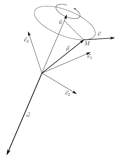
Fig. 2. Rotation of a solid - left coordinate system

The body does not care in which coordinate system we consider it. It rotates the same way it rotated. But the positive direction of reference of the angles of rotation in the new system is clockwise. So, with the existing direction of rotation of the body, the angle of its rotation decreases and $\ dot \ varphi & gt; 0$ , means the vector of angular velocity, according to (9) changes the direction to the opposite.

What will happen to the speed of the body point? And nothing - now, in accordance with (10), the vector will be directed to where the shortest turn from the angular velocity to the radius vector will look going in a clockwise direction, because such a positive direction is chosen in the new coordinate system. So the direction of the velocity vector of the body point will remain the same.

It turns out that during the transition from the right coordinate system to the left and vice versa, that is, when the orientation of the base changes, the angular velocity vector changes direction. So, as a complete geometric object, it is not invariant to a change of base. Such vectors are called pseudovectors . They are also called axial vectors , which emphasizes the fact that the direction of the vector is determined by the positive direction of rotation selected in this coordinate system.

The velocity vector, on the contrary, does not change direction when the orientation of the base changes and is called a true or polar vector.

The result of the vector product of true vectors is the axial vector. But why (10) gives a true vector? Because one of the arguments is an axial vector, and changing its direction when moving to the left coordinate system eliminates the change in the direction of the vector product. Thus, the vector product of the pseudovector and the true vector gives the true vector as output.

In this sense, the angular velocity vector value is somewhat inconvenient. Therefore, when deriving tensor relations of solid mechanics, it is better to rely on the angular velocity tensor, which is invariant with respect to arbitrary transformations of the coordinate system.

3. A bit of practice - the derivation of Euler's kinematic equations from the angular velocity tensor

So that the reader does not get bored of the cumbersome formulas and understand the practical value of the relations obtained, I will give an example of how you can get the expression for the components of the angular velocity through arbitrary parameters of body rotation. For example, through the corners of Euler.

We will work in the Cartesian right coordinate system. Euler angles allow you to set an arbitrary orientation of a solid body in space, as shown in Figure 3.

Fig. 3. Euler angles - sequential rotation of a connected coordinate system around the z, x, z axes

Arbitrary orientation of the body can be obtained by three successive rotations - around the z axis at an angle $\ psi$ (nutation angle), then, around the new position of the x axis at an angle $\ theta$ (precession angle), and, around the new position of the z axis at an angle $\ varphi$ - own rotation angle.

So, the rotation matrix, in Cartesian coordinates, will look like a composition of linear transformations of rotation around the z, x, z axes

$\ mathbf {B} = \ begin {bmatrix} \ cos \ psi & amp; & amp; - \ sin \ psi & amp; & amp; 0 \\ \ sin \ psi & amp; & amp; \ cos \ psi & amp; & amp; 0 \\ 0 & amp; & amp; 0 & amp; & amp; 1 \ end {bmatrix} \ begin {bmatrix} 1 & amp; & amp; 0 & amp; & amp; 0 \\ 0 & amp; & amp; \ cos \ theta & amp & & amp; - \ sin \ theta \\ 0 & amp; & amp; \ sin \ theta & amp; & amp; \ cos \ theta \ end {bmatrix} \ begin {bmatrix} \ cos \ varphi & amp; & amp; - \ sin \ varphi & amp; & amp; 0 \\ \ sin \ varphi & amp; & amp; \ cos \ varphi & amp; & amp; 0 \\ 0 & amp; & amp; 0 & amp; & amp; 1 \ end {bmatrix} =$

$= \ begin {bmatrix} \ cos \ psi \, \ cos \ varphi - \ sin \ psi \ cos \ theta \ sin \ varphi & &; - \ cos \ psi \, \ sin \ varphi - \ sin \ psi \ cos \ theta \ cos \ varphi & &; \ sin \ psi \ sin \ theta \\ \ sin \ psi \, \ cos \ varphi + \ cos \ psi \ cos \ theta \ sin \ varphi & amp; - \ sin \ psi \, \ sin \ varphi + \ cos \ psi \ cos \ theta \ cos \ varphi & &; - \ cos \ varphi \ sin \ theta \\ \ sin \ theta \ sin \ varphi & amp; & amp; \ sin \ theta \ cos \ varphi & amp; & amp; \ cos \ theta \ end {bmatrix} \ quad (11)$

Now we apply one of their expressions to (11) to obtain the rotation tensor

$\ Omega = \ mathbf {g} \ cdot \ mathbf {B} ^ {- 1} \ cdot \ mathbf {\ dot B} = \ mathbf {B} ^ {T} \ cdot \ mathbf {g} \ cdot \ mathbf {\ dot B} = \ mathbf {B} ^ {T} \ cdot \ mathbf {\ dot B}$

Since we are working in the Cartesian basis, the metric tensor is represented by the unit matrix. Performing differentiation and matrix multiplication using SKA , for example in Maple using such commands

 restart; <p>with(LinearAlgebra):</p> <p>A01 := Matrix( [ [cos(psi(t)), -sin(psi(t)), 0], [sin(psi(t)), cos(psi(t)), 0], [0, 0, 1] ]);</p> <p>A12 := Matrix( [ [1, 0, 0], [0, cos(theta(t)), -sin(theta(t))], [0 ,sin(theta(t)), cos(theta(t))] ]);</p> <p>A23 := Matrix( [ [cos(phi(t)), -sin(phi(t)), 0], [sin(phi(t)), cos(phi(t)), 0], [0, 0, 1] ]);</p> <p>B := A01 . A12 . A23;</p> <p>dBdt := map(diff, B, t);</p> <p>Omega := map(simplify,B^(-1) . dBdt, trig);</p>

we get the rotation tensor matrix

$\ Omega = \ begin {bmatrix} 0 & amp; & amp; - \ dot \ varphi - \ dot \ psi \ cos \ theta & amp; & amp; \ dot \ psi \ sin \ theta \ cos \ varphi - \ dot \ theta \ sin \ varphi \\ \ dot \ varphi + \ dot \ psi \ cos \ theta & amp; 0 & amp; & amp; - \ dot \ psi \ sin \ theta \ sin \ varphi - \ dot \ theta \ cos \ varphi \\ - \ dot \ psi \ sin \ theta \ cos \ varphi + \ dot \ theta \ sin \ varphi & &; \ dot \ psi \ sin \ theta \ sin \ varphi + \ dot \ theta \ cos \ varphi & amp; 0 \ end {bmatrix} \ quad (12)$

From (12) it is easy to obtain the components of the angular velocity in the coordinate system associated with the body

$\ omega_x = \ dot \ psi \ sin \ theta \ sin \ varphi + \ dot \ theta \ cos \ varphi \ quad (13)$

$\ omega_y = \ dot \ psi \ sin \ theta \ cos \ varphi - \ dot \ theta \ sin \ varphi \ quad (14)$

$\ omega_z = \ dot \ varphi + \ dot \ psi \ cos \ theta \ quad (15)$

The reader experienced in mechanics will certainly recognize in (13) - (15) the Euler kinematic equations connecting the angular velocity vector with the parameters of body rotation, for which Euler angles are chosen.

Similarly, you can associate the angular velocity with any parameters of rotation. We have done all the transformations to obtain formula (8) in general form, associating the angular velocity with the parameters of the final rotation. But neither the representation (8) nor the representation (13) - (15) is inconvenient for dynamic analysis of the motion of a rigid body, since the above formulas are subject to degeneration at certain values of the parameters. In the sequel, we use (8) to go to the angular velocity expressed through the components of the quaternion not subject to degeneration. And this example is verifiable and illustrative.

Conclusion

This note for the most part - work on the mistakes and inaccuracies made in previous publications. But the result is achieved - we got the definition of the vector of the angular velocity of the body through the parameters of the final rotation and clearly showed that the angular velocity is a pseudovector.

Thanks for attention!

To be continued…

Source: https://habr.com/ru/post/262957/

All Articles