The magic of tensor algebra: Part 7 - The final rotation of a rigid body. Rotation tensor properties and method for calculating it

Content

Introduction

In this article we will continue the topic begun by the previous publication . Last time we, using tensors, revealed the nature of the angular velocity and obtained equations of a general form, allowing it to be calculated. We came to the conclusion that it is naturally derived from the rotation operator of the body-related coordinate system.

And what's inside this operator? For the case of Cartesian coordinates, it is easy to obtain rotation matrices and it is easy to detect their properties by associating with them some method of describing the orientation of the body, for example, the Euler or Krylov angles. Or the vector and the angle of the final rotation. Or quaternion. But this is for Cartesian coordinates.
')
Starting to talk about tensors, we renounced Cartesian coordinates. So good is the tensor notation, because it allows you to make equations for any convenient coordinate system, without focusing on its properties. And the problem is that for, for example, oblique coordinates, the rotation matrix, even for a plane case, is extremely complex. I had enough to check their appearance for a simple turn in the plane.

So the task of this article is to look at its properties without looking inside the rotation tensor and obtain a tensor relation for its calculation. And once the task is set, we will begin to solve it.

1. Properties of the rotation coordinate system tensor

In order to return to the mechanics of a free rigid body, it is necessary to understand what the rotation tensor is. The properties of a tensor are determined by the set of its components and the ratio between them. Since the turning tensor is a second-rank tensor and its components are represented by a matrix, then, not to the detriment of the general theme of the cycle, I will lead the presentation of this section using the term “matrix”. The usual “pointless” notation of the matrix product will be written with a dot, because in the framework of the algebra of tensors we are dealing with a combination of a tensor product with convolution. However, a reservation is also needed here - having criticized myself for the incorrect use of the term "convolution", I missed the moment that under the convolution is often understood its combination with tensor multiplication. At the same time they say, for example, “we turn the vector with the Levi-Civita tensor and we get ...”, meaning just the operation of the inner product.

So, consider the main properties of the rotation matrix $\ mathbf {B}$

The transformation of the rotation of the metric tensor is the identity transformation

$\ mathbf {B} ^ T \ cdot \ mathbf {g} \ cdot \ mathbf {B} = \ mathbf {g}$
The determinant of the rotation matrix is equal to one

$\ det \ mathbf {B} = \ pm 1$
The inverse transform matrix is similar to the transposed direct transform matrix.

$\ mathbf {B} ^ {- 1} = \ mathbf {g} ^ {- 1} \ cdot \ mathbf {B} ^ T \ cdot \ mathbf {g}$
If a $\ det \ mathbf {B} = 1$ , the matrix of algebraic complements and the union matrix constructed from $\ mathbf {B}$ similar to this and its transposed matrix, and the similarity transformation is the metric tensor

$\ mathbf {\ hat {B}} = \ mathbf {g} \ cdot \ mathbf {B} \ cdot \ mathbf {g} ^ {- 1}$

$\ mathop {\ rm adj} \ mathbf {B} = \ mathbf {g} ^ {- 1} \ cdot \ mathbf {B} \ cdot \ mathbf {g}$

The consequence of this property is the equality of traces of the listed matrices.

$\ mathop {\ rm tr} \ mathbf {B} = \ mathop {\ rm tr} \ mathbf {\ hat B} = \ mathop {\ rm tr} \ left (\ mathop {\ rm adj} \ mathbf {B} \ right)$
If a $\ det \ mathbf {B} & gt; 0$ then the eigenvalues of the rotation matrix are equal to unity and have the form

$\ lambda_1 = 1, \ quad \ lambda_ {2,3} = e ^ {\ pm \, i \, \ varphi}$

Where $\ cos \ varphi = \ cfrac {s-1} {2}, \ quad s = \ mathop {\ rm tr} \ mathbf {B}$
If a $\ mathbf {u}$ Is the eigenvector of the rotation matrix corresponding to the complex eigenvalue, then the following relation is true

$\ mathbf {u} ^ T \ cdot \ mathbf {g} \ cdot \ mathbf {u} = 0$

Corollary: real and imaginary parts of an eigenvector $\ mathbf {u}$ corresponding to a complex eigenvalue are orthogonal vectors

$\ mathbf {u} _ {\, r} ^ T \ cdot \ mathbf {g} \ cdot \ mathbf {u} _ {\, i} = 0$

Where $\ mathbf {u} = \ mathbf {u} _ {\, r} + i \, \ mathbf {u} _ {\, i}$ .

I will not give evidence of the properties in the main text - the article already promises to be voluminous. These proofs are not too complicated, but for those interested in them, the following spoiler is made.

Proof of properties 1 - 6 for the inquisitive and meticulous reader

Properties 1 and 3 we proved in the previous article . Property 2 is proved from property 1 trivially, based on the properties of the determinant of the matrix product

$\ det \ mathbf {B} ^ T \, g \ det \ mathbf {B} = g$

$\ left (\ det \ mathbf {B} \ right) ^ 2 = 1$

$\ det \ mathbf {B} = \ pm \, 1$

Property 4 follows from the analytical method for calculating the inverse matrix. $\ det \ mathbf {B} = 1$ then

$\ mathbf {B} ^ {- 1} = \ frac {1} {\ det \ mathbf {B}} \, \ mathop {\ rm adj} \ mathbf {B} = \ mathop {\ rm adj} \ mathbf { B}$

$\ mathop {\ rm adj} \ mathbf {B} = \ mathbf {g} ^ {- 1} \ cdot \ mathbf {B} ^ T \ cdot \ mathbf {g}$

Where $\ mathop {\ rm adj} \ mathbf {B}$ - union matrix (transposed matrix of algebraic complements). Transposing (1), using the symmetry of the metric tensor, we obtain

$\ mathbf {\ hat B} = \ left (\ mathbf {g} ^ {- 1} \ cdot \ mathbf {B} \ cdot \ mathbf {g} \ right) ^ T$

$\ mathbf {\ hat B} = \ mathbf {g} \ cdot \ left (\ mathbf {g} ^ {- 1} \ cdot \ mathbf {B} ^ T \ right) ^ T$

$\ mathbf {\ hat B} = \ mathbf {g} \ cdot \ mathbf {B} \ cdot \ mathbf {g} ^ {- 1}$

Where $\ mathbf {\ hat B}$ - a matrix composed of algebraic complements of the rotation matrix. Relations (1) and (2) are similarity relations. The traces of such matrices are the same.

$\ mathop {\ rm tr} \ mathbf {\ hat B} = \ mathop {\ rm tr} \ left (\ mathop {\ rm adj} \ mathbf {B} \ right) = \ mathop {\ rm tr} \ mathbf {B}$

Let us prove property 5. Let $\ lambda$ - eigenvalue of the rotation matrix to which the eigenvector corresponds $\ mathbf {u}$ . Then

$\ mathbf {B} \ cdot \ mathbf {u} = \ lambda \, \ mathbf {u}$

Multiply this expression by the inverse transform matrix on the left.

$\ mathbf {u} = \ lambda \, \ mathbf {B} ^ {- 1} \ cdot \ mathbf {u}$

subject to property 3

$\ mathbf {u} = \ lambda \, \ mathbf {g} ^ {- 1} \ cdot \ mathbf {B} ^ T \ cdot \ mathbf {g} \ cdot \ mathbf {u}$

We perform complex conjugation, given that the rotation matrix and the metric tensor have real components and their conjugation is reduced to transposition

$\ mathbf {u} ^ {*} = \ overline \ lambda \ left (\ mathbf {g} ^ {- 1} \ cdot \ mathbf {B} ^ T \ cdot \ mathbf {g} \ cdot \ mathbf {u} \ right) ^ {*}$

$\ mathbf {u} ^ {*} = \ overline \ lambda \, \ mathbf {u} ^ {*} \ cdot \ left (\ mathbf {g} ^ {- 1} \ cdot \ mathbf {B} ^ T \ cdot \ mathbf {g} \ right) ^ {T}$

$\ mathbf {u} ^ {*} = \ overline \ lambda \, \ mathbf {u} ^ {*} \ cdot \ mathbf {g} \ cdot \ mathbf {B} \ cdot \ mathbf {g} ^ {- 1 }$

The last expression is multiplied on the right $\ mathbf {g} \ cdot \ mathbf {u}$

$\ mathbf {u} ^ {*} \ cdot \ mathbf {g} \ cdot \ mathbf {u} = \ overline \ lambda \, \ mathbf {u} ^ {*} \ cdot \ mathbf {g} \ cdot \ mathbf {B} \ cdot \ mathbf {u}$

$\ mathbf {u} ^ {*} \ cdot \ mathbf {g} \ cdot \ mathbf {u} = \ overline \ lambda \, \ lambda \, \ mathbf {u} ^ {*} \ cdot \ mathbf {g} \ cdot \ mathbf {u}$

Finally we have the equation

$\ left (1 - \ overline \ lambda \, \ lambda \ right) \ mathbf {u} ^ {*} \ cdot \ mathbf {g} \ cdot \ mathbf {u} = 0$

which is valid only when

$\ overline \ lambda \, \ lambda = \ left | \ lambda \ right | ^ 2 = 1$

i.e

$\ left | \ lambda \ right | = 1$

To calculate the eigenvalues we make the characteristic equation

$\ det \ left (\ mathbf {B} - \ lambda \, \ mathbf {E} \ right) = 0$

calculating the determinant, we arrive at the general form of this equation (for a matrix of dimension (3 x 3))

$\ lambda ^ 3 - \ mathop {\ rm tr} \ mathbf {B} \, \ lambda ^ 2 + \ mathop {\ rm tr} \ mathbf {\ hat B} \, \ lambda - \ det \ mathbf {B} = 0 \ quad (3)$

Enter the notation $s = \ mathop {\ rm tr} \ mathbf {B} = \ mathop {\ rm tr} \ mathbf {\ hat B}$

$\ lambda ^ 3 - s \, \ lambda ^ 2 + s \, \ lambda - 1 = 0 \ quad (4)$

We decompose (4) into factors

$\ left (\ lambda - 1 \ right) \ left (\ lambda ^ 2 + \ lambda + 1 \ right) - s \, \ lambda \ left (\ lambda - 1 \ right) = 0$

$\ left (\ lambda - 1 \ right) \ left (\ lambda ^ 2 - \ lambda \ left (s - 1 \ right) + 1 \ right) = 0$

where we immediately get

$\ lambda _ {\, 1} = 1$

The remaining pair of roots is found by solving a quadratic equation

$\ lambda_ {2,3} = \ frac {s-1} {2} \ pm \ sqrt {\ left (\ frac {s-1} {2} \ right) ^ 2 - 1}$

We introduce a replacement

$\ cos \ varphi = \ frac {s-1} {2}$

which is legitimate, because, putting the roots, in the general case complex-conjugate, according to the Vieta theorem, we have

$\ lambda_2 + \ lambda_3 = s-1$

$2 \, \ mathop {\ rm Re} (\ lambda_2) = s-1$

or by absolute value

$2 \, \ left | \ mathop {\ rm Re} (\ lambda_2) \ right | = \ left | s-1 \ right |$

Because $\ left | \ mathop {\ rm Re} (\ lambda_2) \ right | \ le \ left | \ lambda_2 \ right | = 1$

then obviously

$\ left | s-1 \ right | \ le 2$

Making the replacement, we finally calculate

$\ lambda_ {2,3} = \ cos \ varphi \ pm i \, \ sin \ varphi = e ^ {\ pm \, i \, \ varphi}$

The proof of property 6 will be carried out based on the expression

$\ mathbf {u} = \ lambda \, \ mathbf {g} ^ {- 1} \ cdot \ mathbf {B} ^ T \ cdot \ mathbf {g} \ cdot \ mathbf {u}$

obtained in the proof of equality to a unit of modulus of an eigenvalue. Now, instead of complex conjugation, we transpose it, taking into account the properties of the transposition of the matrix multiplication

$\ mathbf {u} ^ T = \ lambda \, \ mathbf {u} ^ T \ cdot \ mathbf {g} \ cdot \ mathbf {B} \ cdot \ mathbf {g} ^ {{1}$

Multiply the resulting expression by $\ mathbf {g} \ cdot \ mathbf {u}$ on right

$\ mathbf {u} ^ T \ cdot \ mathbf {g} \ cdot \ mathbf {u} = \ lambda \, \ mathbf {u} ^ T \ cdot \ mathbf {g} \ cdot \ mathbf {B} \ cdot \ mathbf {u}$

$\ mathbf {u} ^ T \ cdot \ mathbf {g} \ cdot \ mathbf {u} = \ lambda \, \ lambda \, \ mathbf {u} ^ T \ cdot \ mathbf {g} \ cdot \ mathbf {u }$

Now multiply the resulting equation by the number of complex conjugate eigenvalue, given that its modulus is equal to one

$\ overline \ lambda \, \ mathbf {u} ^ T \ cdot \ mathbf {g} \ cdot \ mathbf {u} = \ overline \ lambda \, \ lambda \, \ lambda \, \ mathbf {u} ^ T \ cdot \ mathbf {g} \ cdot \ mathbf {u}$

$\ overline \ lambda \, \ mathbf {u} ^ T \ cdot \ mathbf {g} \ cdot \ mathbf {u} = \ lambda \, \ mathbf {u} ^ T \ cdot \ mathbf {g} \ cdot \ mathbf {u}$

Finally we arrive at the equation

$\ left (\ lambda - \ overline \ lambda \ right) \, \ mathbf {u} ^ T \ cdot \ mathbf {g} \ cdot \ mathbf {u} = 0$

in which the bracket, due to the complexity of the eigenvalue, is not equal to zero, since

$\ lambda - \ overline \ lambda = 2 \, i \, \ mathop {\ rm Im} (\ lambda)$

Then fair

$\ mathbf {u} ^ T \ cdot \ mathbf {g} \ cdot \ mathbf {u} = 0$

The corollary of this property is proved by simple multiplication.

$\ mathbf {u} ^ T \ cdot \ mathbf {g} \ cdot \ mathbf {u} = \ left (\ mathbf {u} _ {\, r} + i \, \ mathbf {u} _ {\, i } \ right) ^ T \ cdot \ mathbf {g} \ cdot \ left (\ mathbf {u} _ {\, r} + i \, \ mathbf {u} _ {\, i} \ right) = \ left (\ mathbf {u} _ {\, r} ^ T + i \, \ mathbf {u} _ {\, i} ^ T \ right) \ cdot \ mathbf {g} \ cdot \ left (\ mathbf {u } _ {\, r} + i \, \ mathbf {u} _ {\, i} \ right) =$

$= \ mathbf {u} _ {\, r} ^ T \ cdot \ mathbf {g} \ cdot \ mathbf {u} _ {\, r} - \ mathbf {u} _ {\, i} ^ T \ cdot \ mathbf {g} \ cdot \ mathbf {u} _ {\, i} + 2 \, i \, \ mathbf {u} _ {\, r} ^ T \ cdot \ mathbf {g} \ cdot \ mathbf { u} _ {\, i} = 0$

Equating real and imaginary parts to zero

$\ mathbf {u} _ {\, r} ^ T \ cdot \ mathbf {g} \ cdot \ mathbf {u} _ {\, r} - \ mathbf {u} _ {\, i} ^ T \ cdot \ mathbf {g} \ cdot \ mathbf {u} _ {\, i} = 0$

$\ mathbf {u} _ {\, r} ^ T \ cdot \ mathbf {g} \ cdot \ mathbf {u} _ {\, i} = 0$

The last equations imply the required orthogonality and equality of the modules. $\ mathbf {u} _ {\, r}$ and $\ mathbf {u} _ {\, i}$

Why do we need to know about the properties of the rotation tensor?

First, I have completely formulated them, so that the reader can see how the rotation matrix of the curvilinear coordinate system differs from the rotation matrix of the Cartesian system. Practically nothing more, the properties of these matrices are similar. If in the above expressions we put the matrix of the metric tensor of the unit matrix, then we obtain the property of an orthogonal rotation matrix, about which one can read, for example, D.Yu. Pogorelov . Actually this book told me where to dig, to consider the task in general.

Secondly, and this is important, we will prove that the eigenvectors and eigenvalues of these matrices have a mechanical meaning. First we prove the lemma

Let be $\ mathbf {u} _ {\, 1}$ Is the eigenvector corresponding to the real eigenvalue of the rotation tensor, and $\ mathbf {u} _ {\, 1}$ - complies $\ lambda_2 = e ^ {\, i \, \ varphi}$ , and $\ varphi \ ne 0, \, \ pi$ . Let, also, vectors $\ mathbf {u} _ {\, 2 \, r}$ and $\ mathbf {u} _ {\, 2 \, i}$ real and imaginary part $\ mathbf {u} _ {\, 2}$ . Then vectors $\ mathbf {u} _ {\, 1}$ , $\ mathbf {u} _ {\, 2 \, r}$ and $\ mathbf {u} _ {\, 2 \, i}$ form a trio of orthogonal vectors

Property 6 already tells us about orthogonality. $\ mathbf {u} _ {\, 2 \, r}$ and $\ mathbf {u} _ {\, 2 \, i}$ . We now prove that

$\ mathbf {u} _ {\, 1} ^ T \ cdot \ mathbf {g} \ cdot \ mathbf {u} _ {\, 2} = 0 \ quad (1)$

By defining eigenvectors

$\ mathbf {B} \ cdot \ mathbf {u} _ {\, 1} = \ mathbf {u} _ {\, 1} \ quad (2)$

$\ mathbf {B} \ cdot \ mathbf {u} _ {\, 2} = \ lambda_2 \, \ mathbf {u} _ {\, 2} \ quad (3)$

Multiply (3) on the left by $\ mathbf {u} _ {\, 1} ^ T \ cdot \ mathbf {g}$ and transform

$\ mathbf {u} _ {\, 1} ^ T \ cdot \ mathbf {g} \ cdot \ mathbf {B} \ cdot \ mathbf {u} _ {\, 2} = \ lambda_2 \, \ mathbf {u} _ {\, 1} ^ T \ cdot \ mathbf {g} \ cdot \ mathbf {u} _ {\, 2}$

$\ left (\ left (\ mathbf {g} \ cdot \ mathbf {B} \ right) ^ T \ cdot \ mathbf {u} _ {\, 1} \ right) ^ T \ cdot \ mathbf {u} _ { \, 2} = \ lambda_2 \, \ mathbf {u} _ {\, 1} ^ T \ cdot \ mathbf {g} \ cdot \ mathbf {u} _ {\, 2}$

$\ left (\ mathbf {B} ^ T \ cdot \ mathbf {g} \ cdot \ mathbf {u} _ {\, 1} \ right) ^ T \ cdot \ mathbf {u} _ {\, 2} = \ lambda_2 \, \ mathbf {u} _ {\, 1} ^ T \ cdot \ mathbf {g} \ cdot \ mathbf {u} _ {\, 2}$

Given property 3 we can say that

$\ mathbf {g} \ cdot \ mathbf {B} ^ {- 1} = \ mathbf {B} ^ T \ cdot \ mathbf {g} \ quad (5)$

In addition, from (2) directly follows

$\ mathbf {u} _ {\, 1} = \ mathbf {B} ^ {- 1} \ cdot \ mathbf {u} _ {\, 1} \ quad (6)$

Given (6) and (5) we convert (4)

$\ left (\ mathbf {g} \ cdot \ mathbf {u} _ {\, 1} \ right) ^ T \ cdot \ mathbf {u} _ {\, 2} = \ lambda_2 \, \ mathbf {u} _ {\, 1} ^ T \ cdot \ mathbf {g} \ cdot \ mathbf {u} _ {\, 2}$

$\ mathbf {u} _ {\, 1} ^ T \ cdot \ mathbf {g} \ cdot \ mathbf {u} _ {\, 2} = \ lambda_2 \, \ mathbf {u} _ {\, 1} ^ T \ cdot \ mathbf {g} \ cdot \ mathbf {u} _ {\, 2}$

$\ left (1 - \ lambda_2 \ right) \ mathbf {u} _ {\, 1} ^ T \ cdot \ mathbf {g} \ cdot \ mathbf {u} _ {\, 2} = 0$

The expression in parentheses is a nonzero complex number. Assertion (1) is true and the vectors under consideration form an orthogonal triple.

The lemma proved by us is needed to show that the rotation tensor, which we consider in arbitrary coordinates, satisfies the well-known Euler's theorem on finite rotation.

2. Euler's theorem on the final turn

Studying the rotation tensor, we realized that an orthogonal triple of vectors is directly connected with this tensor $\ left (\ vec {u} _ {\, 1}, \ vec {u} _ {, 2 \, r}, \ vec {u} _ {\, 2 \, i} \ right)$ . The first vector in this triple has an interesting property - it does not change when the rotation operator is applied to it. Indeed, after all

$\ mathbf {B} \ cdot \ mathbf {u} _ {\, 1} = \ mathbf {u} _ {\, 1}. \ quad (7)$

This vector remains fixed when turning! And when turning the body, the motionless remains ... the axis of rotation. Means vector $\ vec {u} _ {\, 1}$ sets the orientation in space of the axis of rotation associated with the body of the coordinate system. The Euler theorem, known from the mechanics course, says

For any body that has one fixed current and occupies an arbitrary position in space, there is an axis passing through a fixed point, by rotating around which the body can be moved to any other desired position at the final angle.

Identity (7) gives us a hint about where to look for this axis of rotation - it passes through the eigenvector of the rotation tensor corresponding to its real eigenvalue. Check it out by proving the theorem

The coordinate system associated with the body can be aligned with the base coordinate system by rotating around a vector $\ vec {u} _ {\, 1}$ at an angle $\ varphi$ counterclockwise if the vectors $\ left (\ vec {u} _ {\, 1}, \ vec {u} _ {, 2 \, r}, \ vec {u} _ {\, 2 \, i} \ right)$ form the top three, and at an angle $- \ varphi$ if these vectors form the left three

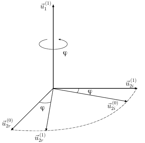
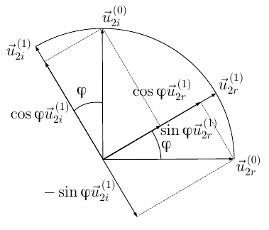
Fig 1. To the proof of the theorem on the final turn

Rotate body-related coordinate system by angle $\ varphi$ around vector $\ vec {u} _ {\, 1}$ . Since the vectors we are considering are orthogonal, the vectors $\ vec {u} _ {\, 2 \, r}$ and $\ vec {u} _ {\, 2 \, r}$ will be rotated in the plane perpendicular to the axis of rotation. Therefore, it is very easy to find the connection between the old position of these vectors in space and the new one (see figure 1)

$\ vec {u} _ {\, 2 \, r} ^ {\, (0)} = \ cos \ varphi \, \ vec {u} _ {\, 2 \, r} ^ {\, (1) } - \ sin \ varphi \, \ vec {u} _ {\, 2 \, i} ^ {\, (1)} \ quad (8)$

$\ vec {u} _ {\, 2 \, i} ^ {\, (0)} = \ sin \ varphi \, \ vec {u} _ {\, 2 \, r} ^ {\, (1) } + \ cos \ varphi \, \ vec {u} _ {\, 2 \, i} ^ {\, (1)} \ quad (9)$

Expressions (8) and (9) are obtained by analyzing the final rotation. On the other hand, the chain of transformations follows from the definition of the eigenvector and the properties of the rotation operator

$\ mathbf {B} \ cdot \ mathbf {u} _ {\, 2} = \ lambda_2 \, \ mathbf {u} _ {\, 2}$

$\ mathbf {B} \ cdot \ mathbf {u} _ {\, 2} = e ^ {\, i \, \ varphi} \, \ mathbf {u} _ {\, 2}$

$\ mathbf {B} \ cdot \ left (\ mathbf {u} _ {\, 2 \, r} + i \ mathbf {u} _ {\, 2 \, i} \ right) = \ left (\ cos \ varphi + i \, \ sin \ varphi \ right) \, \ left (\ mathbf {u} _ {\, 2 \, r} + i \ mathbf {u} _ {\, 2 \, i} \ right)$

$\ mathbf {B} \ cdot \ mathbf {u} _ {\, 2 \, r} + i \, \ mathbf {B} \ cdot \ mathbf {u} _ {\, 2 \, i} = \ cos \ varphi \, \ mathbf {u} _ {\, 2 \, r} - \ sin \ varphi \, \ mathbf {u} _ {\, 2 \, i} + i \ left (\ sin \ varphi \, \ mathbf {u} _ {\, 2 \, r} + \ cos \ varphi \, \ mathbf {u} _ {\, 2 \, i} \ right) \ quad (10)$

Equating the real and imaginary parts (10), we obtain

$\ mathbf {B} \ cdot \ mathbf {u} _ {\, 2 \, r} = \ cos \ varphi \, \ mathbf {u} _ {\, 2 \, r} - \ sin \ varphi \, \ mathbf {u} _ {\, 2 \, i} \ quad (11)$

$\ mathbf {B} \ cdot \ mathbf {u} _ {\, 2 \, i} = \ sin \ varphi \, \ mathbf {u} _ {\, 2 \, r} + \ cos \ varphi \, \ mathbf {u} _ {\, 2 \, i} \ quad (12)$

Comparing (8) and (11), (9) and (12), we conclude that applying the rotation operator to vectors leads to their rotation around the axis $\ vec {u} _1$ at an angle $\ varphi$

I must say, our results look pretty impressive - after all, not knowing about the insides of the rotation tensor, we investigated everything (at least its practically significant properties). And we are not particularly interested in the insides of specific rotation tensors, our main task is to learn how to calculate this tensor, so that it provides a rotation around the axis we need at the required angle

3. Expression of the rotation tensor through the parameters of the final rotation. Rodrigue Formula

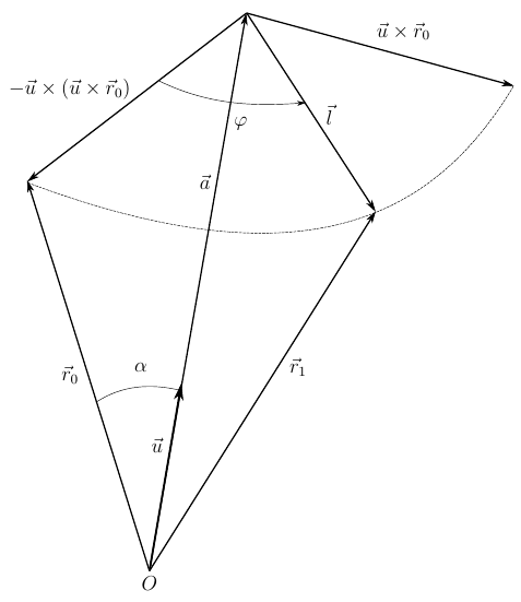
Consider the final rotation of an arbitrary vector. In the base coordinate system, its position corresponds to $\ vec {r} _ {\, 0}$ associated with the body - $\ vec {r} _ {\, 1}$ . The turn takes place at an angle. $\ varphi$ around the axis passing through the vector $\ vec {u}$ which is set to single

$\ left | \ vec {u} \ right | = 1$

Fig. 2. The final rotation of an arbitrary vector

From Figure 2, the vector relationship is obvious.

$\ vec {r} _1 = \ vec {a} + \ vec {l} \ quad (13)$

Where $\ vec {l}$ - vector perpendicular to the axis of rotation, whose length is equal to

$l = r _ {\, 0} \ sin \ alpha$

Vector $\ vec {a}$ directed along the axis of rotation and can be expressed as follows

$\ vec {a} = a \, \ vec {u} = (\ vec {u} \ cdot \ vec {r} _0) \, \ vec {u}$

On the other hand, the following vectors have the same module

$\ left | \ vec {u} \ times \ vec {r} _ {\, 0} \ right | = r _ {\, 0} \ sin \ alpha = l$

$\ left | - \ vec {u} \ times (\ vec {u} \ times \ vec {r} _ {\, 0}) \ right | = l$

mean vector $\ vec {l}$ can be expressed through them

$\ vec {l} = \ cos \ varphi \, \ left (- \ vec {u} \ times (\ vec {u} \ times \ vec {r} _ {\, 0}) \ right) + \ sin \ varphi \, (\ vec {u} \ times \ vec {r} _ {\, 0})$

Now, the written vector relations will be represented in the tensor component form

$a ^ {\, m} = u ^ {\, m} \, g_ {ik} \, u ^ {\, j} \, r ^ {\, k (0)}$

$l ^ {\, m} = - \ cos \ varphi \, \ left (\ varepsilon ^ {\, mqi} \, u _ {\, q} \, \ varepsilon _ {\, ijk} \, u ^ {, j} \, r_0 ^ {\, k} \ right) + \ sin \ varphi \, \ left (g ^ {\, mi} \, \ varepsilon {\, ijk} \, u ^ {\, j} \ , r_0 ^ {\, k} \ right) \ quad (15)$

and we introduce two antisymmetric tensors

$U ^ {\, mi} = \ varepsilon ^ {\, mqi} \, u _ {\, q} \ quad (16)$

$U _ {\, ik} = \ varepsilon _ {\, ijk} \, u ^ {\, j} \ quad (17)$

Given which you can write

$r_1 ^ {\, m} = \ left (u ^ {\, m} \, g_ {ik} \, u ^ {\, j} - \ cos \ varphi \, U ^ {mi} \, U _ {\ , ik} + \ sin \ varphi \, g ^ {mi} \, U_ {ik} \ right) \, r_0 ^ {\, k} \ quad (18)$

Convolution of tensors (16) and (17) on a common index, we execute by writing them through the matrix of components

$\ mathbf {\ tilde U} \ cdot \ mathbf {U} = \ frac {1} {\ sqrt g} \ begin {bmatrix} 0 & amp; -u_3 & amp; & amp; u_2 \\ u_3 & amp; & amp; 0 & amp; & amp; -u_1 \\ -u_2 & amp; & amp; u_1 & amp; & amp; 0 \ end {bmatrix} \ sqrt g \ begin {bmatrix} 0 & amp; & amp; -u ^ 3 & amp; & amp; u ^ 2 \\ u ^ 3 & amp; & amp; 0 & amp; & amp; -u ^ 1 \\ -u ^ 2 & amp; & amp; u ^ 1 & amp; & amp; 0 \ end {bmatrix} = - \ begin {bmatrix} u_3 \, u ^ 3 + u_2 \, u ^ 2 & amp; -u_1 \, u ^ 2 & amp; & amp; -u_1 \, u ^ 3 \\ -u_2 \, u ^ 1 & amp; u_1 \, u ^ 1 + u_3 \, u ^ 3 & amp & amp; -u_2 \, u ^ 3 \\ -u_3 \, u ^ 1 & amp; -u_3 \, u ^ 2 & amp; & amp; u_1 \, u ^ 1 + u_2 \, u ^ 2 \ end {bmatrix} \ quad (19)$

It is easy to see that (19) is equivalent

$U ^ {\, mi} \, U _ {\, ik} = - \ left (\ delta_k ^ {\, m} \ left | u \ right | ^ 2 - u_m \, u ^ {\, k} \ right ) = - \ left (\ delta_k ^ {\, m} - u ^ j \, g_ {jm} \, u ^ {\, k} \ right) \ quad (20)$

Convert (18) with (20)

$r_1 ^ {\, m} = \ left [u ^ {\, m} \, g_ {jk} \, u ^ {\, j} - \ cos \ varphi \, u ^ {\, j} \, g_ {jk} \, u ^ {\, m} + \ cos \ varphi \, \ delta_k ^ {\, m} + \ sin \ varphi \, g ^ {mi} \, U_ {ik} \ right] \, r_0 ^ {\, k} \ quad (21)$

From (21) we obtain the expression for the rotation operator

$B_k ^ {\, m} = u ^ {\, m} \, g_ {jk} \, u ^ {\, j} - \ cos \ varphi \, u ^ {\, j} \, g_ {jk} \, u ^ {\, m} + \ cos \ varphi \, \ delta_k ^ {\, m} + \ sin \ varphi \, g ^ {mi} \, U_ {ik} \ right \ quad (22)$

Where

$U_ {ik} = \ varepsilon_ {ijk} \, r ^ {\, j}$

- antisymmetric tensor of rank (0,2), generated by the ort of the axis of rotation.

or, in component form

$\ mathbf {B} = \ mathbf {u} \ cdot \ mathbf {u} ^ T \ cdot \ mathbf {g} - \ cos \ varphi \, \ mathbf {g} \ cdot \ mathbf {u} \ cdot \ mathbf {u} ^ T + \ cos \ varphi \, \ mathbf {E} + \ sin \ varphi \, \ mathbf {g} ^ {- 1} \ cdot \ mathbf {U} \ quad (23)$

Expressions (22) and (23) are called the Rodrigues rotation formula. We obtain them for a coordinate system with an arbitrary nondegenerate metric.

Conclusion

All of the above was considered for one single purpose - to obtain the expression of the rotation operator for an arbitrary coordinate system. This will allow us to express through (23) the tensor and pseudovector of angular velocity, and then angular acceleration. After this, we will choose the parameters characterizing the orientation of the solid in space (these will be Rodrig – Hamilton parameters, yes, we will talk about quaternions) and we will write down the equations of motion of a solid body in generalized coordinates. , , , .

Thanks for attention!

To be continued…

Source: https://habr.com/ru/post/262263/

All Articles