The magic of tensor algebra: Part 6 - Kinematics of a free solid. Nature of angular velocity

Content

Introduction

What is angular velocity? Scalar or vector value? In fact, this is not an idle question.

In lectures on theoretical mechanics at the university, I, following the traditional method of presenting the kinematics course, introduced the concept of angular velocity in the topic "The velocity of a body point during rotational motion." And there the angular velocity first appears as a scalar, with the following definition.

The angular velocity of a solid is the first derivative of the angle of body rotation with time.
$\ omega = \ frac {d \ varphi} {dt}$

And then, when considering the canonical Euler formula for the velocity of a body point during rotation
')

$\ vec {v} _M = \ vec {\ omega} \ times \ vec {r}$

The following definition is usually given.

The angular velocity of the body is a pseudo-vector directed along the axis of rotation of the body in the direction from which rotation looks counterclockwise.

Another particular definition, which, firstly, asserts the immobility of the axis of rotation, secondly, imposes consideration of only the right coordinate system. Finally, the term “pseudovector” is usually explained to students as follows: “Look, because we have shown that omega is a scalar quantity. And we introduce a vector in order to write out the Euler formula. ”

When considering spherical motion, it turns out that the axis of rotation changes direction, the angular acceleration is directed tangentially to the hodograph of the angular velocity, and so on. Obstacles and introductory assumptions multiply.

Considering the level of schoolchildren’s training, as well as the blatant stupidity allowed in bachelor’s training programs, when theorem begins with the first (think!) Semester, such gradual introductory exercises on sticks, ropes and acorns are probably justified.

But we'll look at what is called the “under the hood” of the problem and, armed with the apparatus of tensor calculus, find out that the angular velocity is a pseudovector generated by an antisymmetric tensor of the second rank.

I think for the seed it is enough, and therefore - let's start!

1. Free movement of a solid body. Rotational tensor

So, as we know from the traditional university course of theorem

If the movement performed by the body is not limited to connections, then such a movement is called free

This is the most common case of body movement. The following figure illustrates the fact that the free movement of the body can be represented as the sum of two movements: translational along with the pole $O_1$ and spherical around the pole.

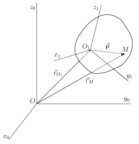
Fig. 1. The usual illustration from the course of theoretical mechanics: determining the position of a free solid body in space.

Let me remind you that this is an absolutely solid body , that is, a body, the distance between the points of which does not change over time. You can also say that a solid body is an immutable mechanical system.

As can be seen from Figure 1, it’s common practice to consider two coordinate systems - one $O \, x_0 \, y_0 \, z_0$ considered fixed and called base , the other $O \, x_1 \, y_1 \, z_1$ rigidly connected with the body and rotated relative to the base with it. This coordinate system is called bound .

At first, I also wanted to restrict myself to Cartesian coordinates. But then my readers would ask me a logical question - “why then are there tensors?”. Therefore, having spent four for agonizing thoughts and “nagulyav” the final decision a couple of hours ago, I decided to wipe at “William, ours, Shakespeare” and set forth further arguments in curvilinear coordinates.

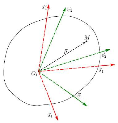
Fig. 2. Orientation of a solid in a local basis.

Let the pole position $Q_1$ set by vector

$q ^ {\, i} = q ^ {\, i} (t)$

Moreover, this vector should not be understood as a radius vector, since in curvilinear coordinates such a concept is meaningless.

At the point O _{1, a} local frame of the base coordinate system is defined, formed by a triplet of vectors $(\ vec {s} _1, \, \ vec {s} _2, \, \ vec {s} _3)$ . A moving frame is associated with a moving body. $(\ vec {e} _1, \, \ vec {e} _2, \, \ vec {e} _3)$ . The rotation of the associated frame relative to the base can be specified by a linear operator. We obtain this operator and investigate its properties.

Consider some point M belonging to the body. You can draw a vector from the pole $\ vec {\ rho}$ fixed relative to the associated frame. It can be expanded by the vectors of this frame.

$\ vec {\ rho} = \ rho ^ {\, i} \ vec {e} _i \ quad (2)$

and on the base reference vectors

$\ vec {\ rho} ^ {\, '} = \ rho ^ {\,' i} \ vec {e} _i \ quad (3)$

Each vector of the associated frame can be expanded through the vectors of the base frame.

$\ vec {e} _i = \ beta_ {i} ^ {\, \, j} \ vec {s} _j$

Substitute (4) into (2) and compare with (3)

$\ rho ^ {\, 'i} \ vec {s} _i = \ rho ^ {i} \ beta_ {i} ^ {\, \, j} \ vec {s} _j \ quad (5)$

From (5) it is clear that the components of the vector $\ vec {\ rho}$ in the base coordinate system, recalculated through its components in the related system by applying a linear operator

$\ rho ^ {\, 'i} = \ rho ^ {i} \ beta_ {i} ^ {\, \, j} \ quad (6)$

or index-free

$\ rho ^ {\, '} = \ mathbf {B} (t) \ cdot \ rho ^ {i} \ quad (6)$

where are the matrix columns

$\ mathbf {B} = \ begin {bmatrix} \ beta_1 ^ {\, \, 1} & amp; & amp; \ beta_2 ^ {\, \, 1} & amp; & amp; \ beta_3 ^ {\, \, 1} \\ \ beta_1 ^ {\, \, 2} & amp; & amp; \ beta_2 ^ {\, \, 2} & amp; & amp; \ beta_3 ^ {\, \, 2} \\ \ beta_1 ^ {\, \, 3} & amp; & amp; \ beta_2 ^ {\, \, 3} & amp; & amp; \ beta_3 ^ {\, \, 3} \ end {bmatrix}$

- contravariant components of the vectors of the associated frame in relation to the base. The point, as we have already noted in the last article , denotes multiplication of tensors with subsequent convolution along the adjacent pair of indices. Linear operator

$\ mathbf {B} = \ mathbf {B} (t) \ quad (7)$

acts on vectors in such a way that rotates them about a certain axis, without changing the length and angle between the vectors. Such a transformation of space is called orthogonal . In order for such a transformation to be possible, operator (7) must have well-defined properties. If the length of the basis vectors and the angles between them do not change, then this means the equality of all pairwise scalar products of the frames of the frame in both the base and the related coordinate systems

$\ vec {e} _ {i} \ cdot \ vec {e} _j = \ vec {s} _i \ cdot \ vec {s} _j \ quad (8)$

The right side of (8) is the local metric tensor

$\ vec {e} _ {i} \ cdot \ vec {e} _j = g_ {ij}$

$g_ {kl} \, \ beta_i ^ {\, \, l} \, \ beta_j ^ {\, \, k} = g_ {ij} \ quad (9)$

$\ mathbf {B} ^ T \ cdot \ mathbf {g} \ cdot \ mathbf {B} = \ mathbf {g} \ quad (10)$

Operator $\ mathbf {B}$ is essentially an ordinary matrix of rotation of the coordinate system. And (10) states that if the transposed rotation matrix is multiplied by the metric tensor, and the result is multiplied by the rotation matrix, we get again the metric tensor. It can be concluded that

Transformation of coordinates when turning is identical for the metric tensor, that is, it translates the metric tensor into itself.

In expression (10), it is easy to see the transformation of the metric tensor about the change of the coordinate system, which we discussed in detail in the very first article of the cycle

Stop! But we know that the rotation matrices are usually orthogonal, that is, the product of the rotation matrix and its transposed gives a unit matrix, in other words, it is enough to transpose it to reverse the rotation matrix.

But orthogonality is characteristic of turning matrices, which transform the orthonormal Cartesian basis. Here we are dealing with a local basis, the rotation of which must preserve the lengths of the vectors and the angles between them. If we take the basis as Cartesian, then from (10) we get the usual properties of the rotation matrix, for example, its orthogonality.

For further calculations, we need to know how the inverse transform matrix will look, that is, $\ mathbf {B} ^ {- 1}$ . Well, let's see. To do this, multiply (10) on the left by $\ mathbf {g} ^ {- 1}$ and to the right of $\ mathbf {B} ^ {- 1}$

$\ mathbf {g} ^ {- 1} \ cdot \ mathbf {B} ^ T \ cdot \ mathbf {g} \ cdot \ mathbf {B} \ cdot \ mathbf {B} ^ {- 1} = \ mathbf {g } ^ {- 1} \ cdot \ mathbf {g} \ cdot \ mathbf {B} ^ {- 1}$

where we immediately get

$\ mathbf {B} ^ {- 1} = \ mathbf {g} ^ {- 1} \ cdot \ mathbf {B} ^ T \ cdot \ mathbf {g}$

It turns out that the inverse transformation matrix is indeed obtained from the transposed transformation matrix, but with the participation of the metric tensor. Expressions (10) and (11) will be very useful to us, but for now we will draw some conclusions.

The law of free motion of a rigid body can be written in curvilinear coordinates in the form of a system of equations

$\ mathbf {q} = \ mathbf {q} (t) \ quad (12)$

$\ mathbf {B} = \ mathbf {B} (t) \ quad (13)$

In this case, (12) is the law of motion of the pole, and (13) is the law of spherical body motion around the pole. At the same time (13) is a rank tensor (1,1), called the rotation tensor .

2. The speed of the point of the body with free movement. Angular velocity goes on stage

We calculate the velocity of the point M , whose position in the associated coordinate system is set constant, by virtue of the hardness of the body, curvilinear coordinates

$\ rho ^ {\, i} = \ mathop {\ rm const}$

From the course of theoretical mechanics, a formula is known that determines the velocity of a point of a body in a given motion.

$\ vec {v} _M = \ vec {v} _ {O_1} + \ vec \ omega \ times \ vec \ rho$

Where $\ vec {v} _ {O_1}$ - pole speed; $\ vec \ omega \ times \ vec \ rho = \ vec {u}$ - the speed of the point around the pole.

Since all coordinates except (13) are defined relative to the base frame, we can write

$q_M ^ {\, (0)) i} = q ^ {(0) \, i} + \ beta_ {j} ^ {\, \, i} \, \ rho ^ {\, (1) j} \ quad (15)$

The index in parentheses means the coordinate system in which the components are taken (0 is basic, 1 is connected). Differentiate (15) by time, taking into account (13)

$\ dot q_M ^ {\, (0) i} = \ dot q ^ {(0) \, i} + \ dot \ beta_ {j} ^ {\, \, i} \, \ rho ^ {\, ( 1) j}$

Let us turn in (16) to the connected coordinate system, multiplying (15) from the left to $\ mathbf {B} ^ {- 1}$

$\ dot q_M ^ {\, (1) i} = \ dot q ^ {(1) \, i} + \ beta_ {k} ^ {\, '\, i} \, \ dot \ beta_ {j} ^ {\, \, k} \, \ rho ^ {\, (1) j} \ quad (17)$

Where $\ beta_ {k} ^ {\, '\, i}$ - component of the inverse transform operator $\ mathbf {B} ^ {- 1}$ .

Now compare (17) and (14). In the last term, the vector product should come out. Recalling the definition of a vector product through the Levi-Civita tensor given in the second article of the cycle, we note that it gives a covector at the output, so in (17) we turn to the covariant components, multiplying this expression by the left-hand metric tensor

$\ dot q_ {Mi} ^ {\, (1)} = \ dot q _ {\, i} ^ {(1)} + g_ {il} \, \ beta_ {k} ^ {\, '\, l} \, \ dot \ beta_ {j} ^ {\, \, k} \, \ rho ^ {\, (1) j} \ quad (18)$

Now let us imagine what the covector of the velocity of a point would look like relative to the plus, written through the angular velocity vector

$u _ {\, i} = \ varepsilon_ {ijk} \, \ omega ^ {\, (1) j} \, \ rho ^ {\, (1) k}$

while noticing that

$\ Omega _ {\, ik} ^ {\, (1)} = \ varepsilon_ {ijk} \, \ omega ^ {\, (1) j}$

the antisymmetric tensor of the second rank, which we talked about in the last article < . Thus, we would prove that

$\ Omega _ {\, ij} = g _ {\, il} \, \ beta_ {k} ^ {\, '\, l} \, \ dot \ beta_ {j} ^ {\, \, k} \ quad ( nineteen)$

is an antisymmetric second-rank tensor. For this, it is necessary to prove that (19) changes its sign during the permutation of indices (transposition). In this case, we will take into account that the metric tensor is an absolutely symmetric second-rank tensor and does not change when transposed. Therefore, we investigate the relationship between the rotation matrices, for which we need expressions (10) and (11). But before proceeding, we prove another auxiliary assertion.

3. Lemma on the covariant derivative of the metric tensor

The covariant derivative of the metric tensor is zero

Let us turn to the concept of a covariant derivative of the vector, which was mentioned in the third article . Then we derived expressions for the contravariant components of the covariant derivative of the vector

$\ nabla_j \, a ^ m = \ left (\ frac {\ partial a ^ m} {\ partial q ^ j} + a ^ i \, \ Gamma_ {ij} ^ m \ right)$

As with any vector, the components of this vector can be transformed into covariant multiplication and convolution with the metric tensor.

$\ nabla_j a_i = g _ {\, im} \, \ nabla_j \, a ^ m \ quad (20)$

And you can differentiate covariant components directly

$\ nabla_j a_i = \ nabla_j \ left (g _ {\, im} \, a ^ m \ right) = \ nabla_j \, g _ {\, im} \, a ^ m + g _ {\, im} \, \ nabla_j \, a ^ m \ quad (21)$

Comparing (21) and (20) we come to the conclusion that equality is possible only if the statement of the lemma is true

$\ nabla_j \, g _ {\, im} = 0 \ quad (22)$

4. Angular velocity as an antisymmetric tensor of the second rank

Now, we rewrite (19) in index-free form, taking into account equation (11)

$\ Omega = \ mathbf {g} \ cdot \ mathbf {B} ^ {- 1} \ cdot \ mathbf {\ dot {B}} = \ mathbf {B} ^ {\, T} \ cdot \ mathbf {g} \ cdot \ mathbf {\ dot {B}} \ quad (23)$

Next, we need a connection between the rotation operator and its derivative — we differentiate (10) with respect to time

$\ mathbf {\ dot {B}} ^ T \ cdot \ mathbf {g} \ cdot \ mathbf {B} + \ mathbf {B} ^ T \ cdot \ mathbf {g} \ cdot \ mathbf {\ dot {B} } + \ mathbf {B} ^ T \ cdot \ frac {\ partial \ mathbf {g}} {\ partial \ mathbf {q}} \, \ mathbf {\ dot {q}} \ cdot \ mathbf {B} = \ frac {\ partial \ mathbf {g}} {\ partial \ mathbf {q}} \, \ mathbf {\ dot {q}}$

or by collecting the derivatives of the metric tensor on the right side

$\ mathbf {\ dot {B}} ^ T \ cdot \ mathbf {g} \ cdot \ mathbf {B} + \ mathbf {B} ^ T \ cdot \ mathbf {g} \ cdot \ mathbf {\ dot {B} } = \ frac {\ partial \ mathbf {g}} {\ partial \ mathbf {q}} \, \ mathbf {\ dot {q}} - \ mathbf {B} ^ T \ cdot \ frac {\ partial \ mathbf {g}} {\ partial \ mathbf {q}} \, \ mathbf {\ dot {q}} \ cdot \ mathbf {B} \ quad (24)$

But, the derivatives of the metric tensor in (24) will be equal to zero, by virtue of the equality to zero of the covariant derivative of the metric tensor. So the right side of (24) is zero

$\ mathbf {\ dot {B}} ^ T \ cdot \ mathbf {g} \ cdot \ mathbf {B} + \ mathbf {B} ^ T \ cdot \ mathbf {g} \ cdot \ mathbf {\ dot {B} } = 0 \ quad (25)$

Using the properties of the transpose operation, we transform (25)

$\ left (\ left (\ mathbf {\ dot {B}} ^ T \ cdot \ mathbf {g} \ cdot \ mathbf {B} \ right) ^ T \ right) ^ T + \ mathbf {B} ^ T \ cdot \ mathbf {g} \ cdot \ mathbf {\ dot {B}} = 0$

$\ left (\ mathbf {B} ^ T \ cdot \ left (\ mathbf {\ dot {B}} ^ T \ cdot \ mathbf {g} \ right) ^ T \ right) ^ T + \ mathbf {B} ^ T \ cdot \ mathbf {g} \ cdot \ mathbf {\ dot {B}} = 0$

$\ left (\ mathbf {B} ^ T \ cdot \ mathbf {g} ^ T \ cdot \ mathbf {\ dot {B}} \ right) ^ T + \ mathbf {B} ^ T \ cdot \ mathbf {g} \ cdot \ mathbf {\ dot {B}} = 0 & quot;$

Because $\ mathbf {g} ^ T = \ mathbf {g}$ and taking into account (23), we obtain

$\ left (\ mathbf {B} ^ T \ cdot \ mathbf {g} \ cdot \ mathbf {\ dot {B}} \ right) ^ T + \ mathbf {B} ^ T \ cdot \ mathbf {g} \ cdot \ mathbf {\ dot {B}} = 0$

$\ Omega ^ T + \ Omega = 0 \ quad (26)$

The antisymmetry of the tensor (19) directly follows from (26)

$\ Omega ^ T = - \ Omega \ quad (26)$

Well, since (19) antisymmetric tensor, then we boldly rewrite (18)

$\ dot q_ {Mi} ^ {\, (1)} = \ dot q _ {\, i} ^ {(1)} + \ Omega _ {\, ij} ^ {(1)} \, \ rho ^ {\ , (1) j} \ quad (28)$

Thus, we conclude that (19) and (23) are nothing more than an antisymmetric angular velocity tensor

5. Angular velocity pseudo vector

Any antisymmetric tensor can be associated with the pseudovector, which we have already received in the previous article. We repeat this result for the angular velocity tensor.

$\ omega ^ {\, j} = \ frac {1} {2} \, \ varepsilon ^ {\, ijk} \, \ Omega _ {\, ik} = \ frac {1} {2} \, \ varepsilon ^ {\, ijk} \, \ beta_i ^ {\, \, p} \, g _ {\, pl} \, \ dot \ beta_k ^ {\, \, l} \ quad (29)$

Perhaps the reader is familiar with the common approach of replacing a vector product by multiplying an skew-symmetric matrix constructed from the first vector according to a certain rule by the second vector. So this rule is obtained in a natural way, if we use tensor calculus as a tool. Indeed, this is the skew-symmetric matrix, which in the matrix presentation of the mechanics replace the angular velocity

$\ Omega = \ sqrt g \, \ begin {bmatrix} 0 & amp; & amp; - \ omega ^ {\, 3} & amp; & amp; \ omega ^ {\, 2} \\ \ omega ^ {\, 3} & amp; & amp; 0 & amp; & amp; - \ omega ^ {\, 1} \\ - \ omega ^ {\, 2} & amp; & amp; \ omega ^ {\, 1} & amp; & amp; 0 \ end {bmatrix}$

Perhaps the attentive reader will see that the signs in the resulting matrix are opposite to what we received in the article devoted to antisymmetric tensors. Yes, that's right, because in that article we folded the vector with the Levi-Civita tensor on its third index k , here we perform the convolution on the average index j, which gives opposite signs.

The matrix (30) is often found in the literature, in particular in the works of D.Yu. Pogorelov , but there it is introduced as a mnemonic rule. Formula (29) gives a clear connection between the angular velocity vector and the skew-symmetric matrix. It also makes it possible to move from (28) to the formula

$\ dot q_ {Mi} ^ {\, (1)} = \ dot q _ {\, i} ^ {(1)} + \ varepsilon _ {\, ijk} \, \ omega ^ {\, (1) j} \ rho ^ {\, (1) k} \ quad (31)$
Which, suddenly, is equivalent to the vector relation

$\ vec {v} _M = \ vec {v} _ {O_1} + \ vec {\ omega} \ times \ vec {\ rho}$

Conclusion

This article had a lot of math. And I’m forced to limit myself to this material for now - the article was published long and saturated with formulas. This topic will be continued and deepened in the next articles of the cycle.

What conclusion can we make now? But what

The angular velocity of a solid is an antisymmetric tensor, or, corresponding to it, a pseudovector generated by the body rotation tensor relative to the base coordinate system

In order to write this work it was necessary to shovel a mountain of literature. The main calculations are made by the author independently. The stumbling block was the rotation matrix for the case of oblique coordinates. I did not immediately discern in relation (10) a transformation that left the metric invariant, although, in view of the previously written articles, it would have followed. Understanding this connection helped me terribly in terms of design, but a very sensible site “What Mathematics Looks Like” . By the way, it is clear that all relations go over into known ones for orthogonal matrices, if the metric tensor is made single.

Talk about solid mechanics will continue, but for now - that's all. Thanks for attention!

To be continued…

Source: https://habr.com/ru/post/262129/

All Articles