Visualization of static and dynamic networks on R, part 1
Very many systems and phenomena are representable in the form of networks, i.e. a set of objects and relationships between them. The network is not only an abstraction, but also an illustrative data visualization tool. You can display the importance of an object, the weight of each connection, indicate the key groups of elements, highlight them and emphasize the connections between them. The main task of visualization is to submit key information about the properties of a system or phenomenon as easy as possible for perception. In the ideal case, system analysis and visualization of its results can be done within a single tool. R with its extensive package of packages allows it.
The main thing when designing a network visualization is the goal to be achieved. What structural properties would we like to highlight?

Network maps are by no means the only graph visualization tool - in some cases, other formats for representing networks are preferable, even simple graphs of key properties.
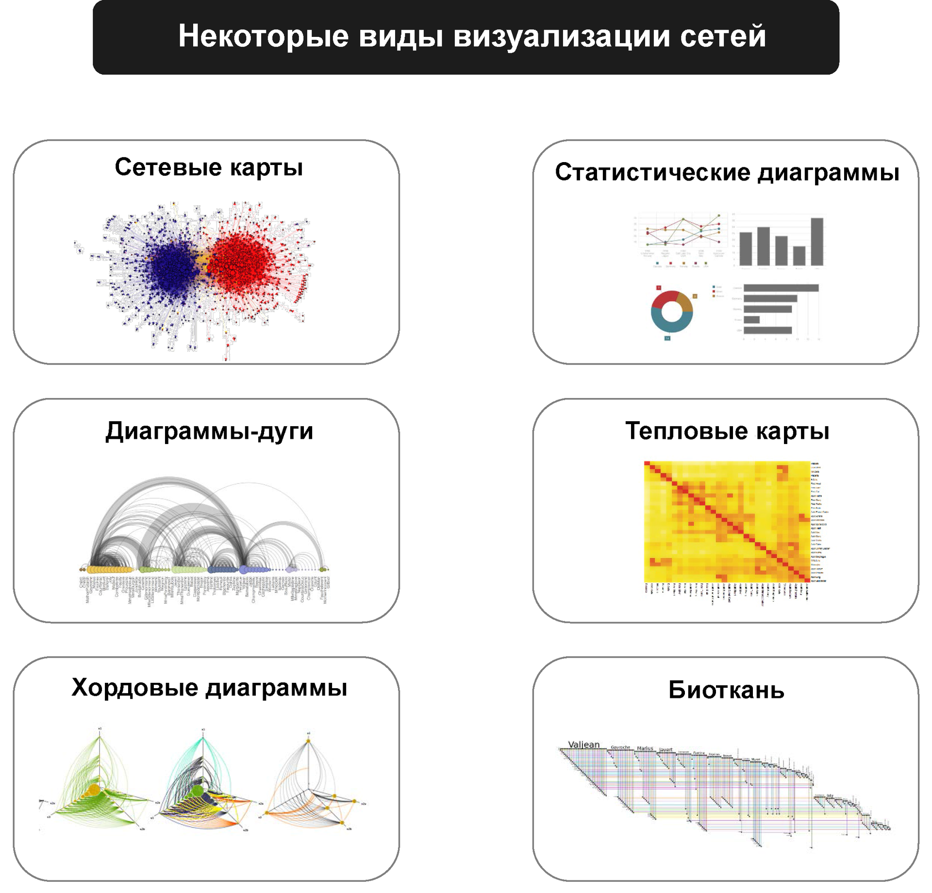
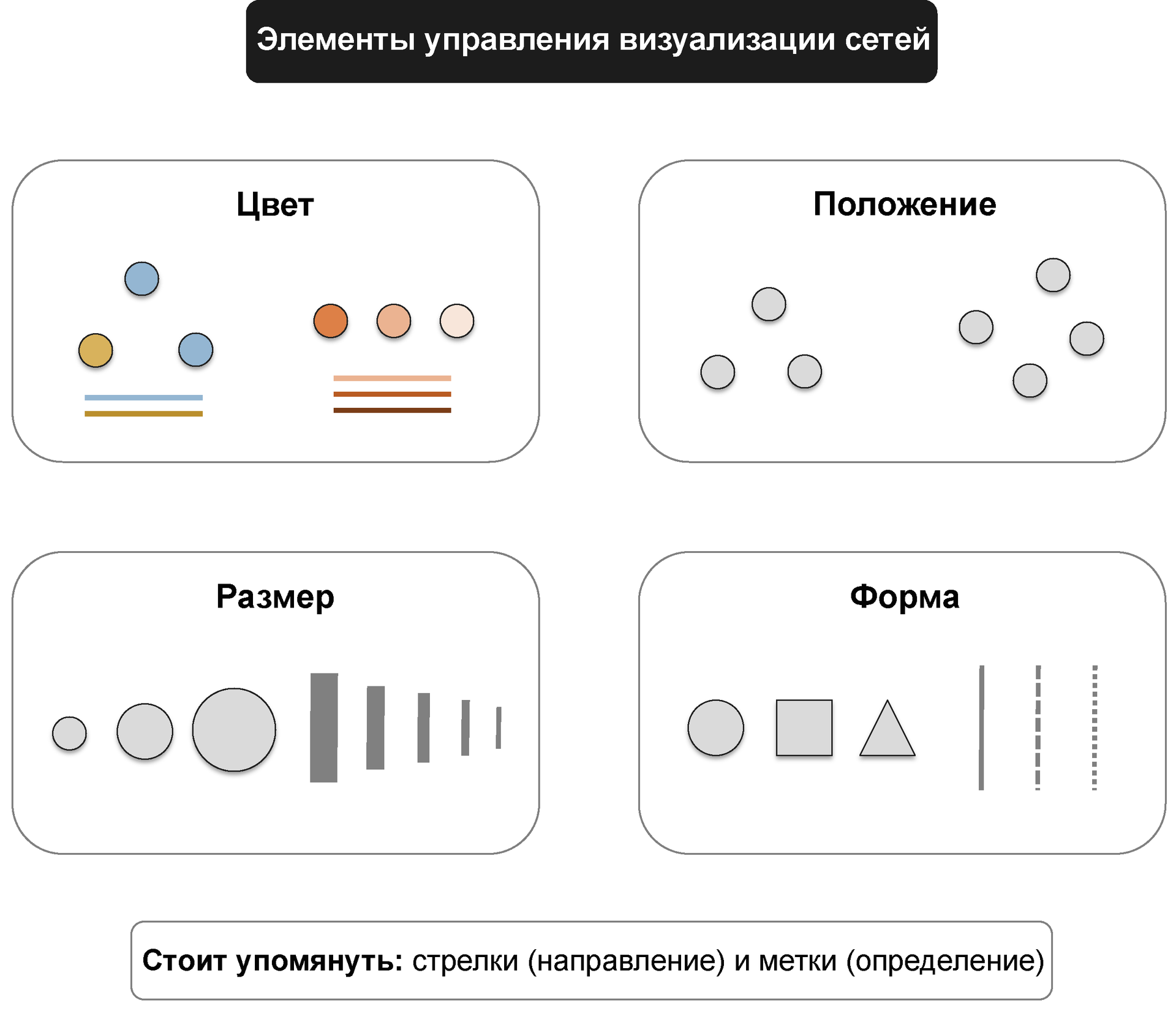
In maps of networks, as well as in other visualization formats, there are several key settings that affect the final result. The main ones are color, size, shape and relative position.
')
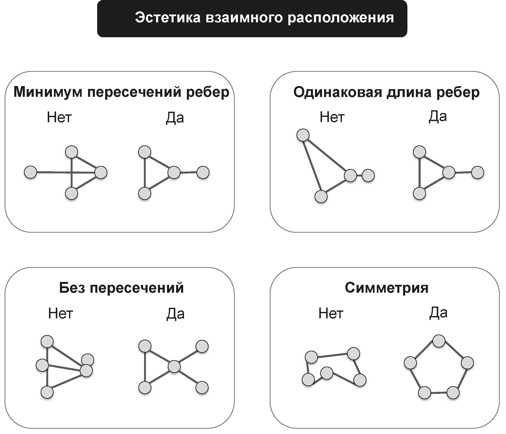
Modern graph views are optimized based on performance requirements and aesthetic considerations. In particular, it is necessary to minimize the overlap and intersection of the edges, to establish the same length of edges in the graph.
In this guide, we will mainly work with two small datasets. Both contain information about the media. One contains a network of hyperlinks and mentions in news resources. Another is a network of links between objects and mass media consumers. Although there is little data in the examples, many of the ideas from the generated visualizations can be extended to medium and large networks. For the same reason, we will rarely use visual tools, for example, the shape of vertex symbols: they are almost impossible to distinguish in large graphs. Moreover, when displaying very large networks, you can even hide edges, since you need to focus on identifying and displaying groups of vertices. Generally speaking, the size of networks that can be visualized with R is limited only by the amount of RAM in your machine. But it should be emphasized that in many cases the visualization of large networks in the form of a giant pom-pom is far less useful than graphs with the key properties of the graph.
This guide uses several key packages that must be installed before proceeding. Some more libraries will be mentioned, but they are optional and can be skipped. The following main libraries will be used - igraph (supported by Gabor Zardi and Tamas Nepush ), sna , network (supported by Carter Butts and the Statnet team ) and ndtv (supported by Sky Bender de Moll ).
The first data set to work with consists of two files: “Media-Example-NODES.csv” and “Media-Example-EDGES.csv” (you can download it here ).
Examine the data:
Please note that there are more edges than unique “from” - “to” combinations. This means that there are cases in the data when there is more than one connection between two vertices. We will roll all the edges of the same type between two nodes, summing their weights using the
Examine the data:
You can verify that the links2 is the mating matrix for a two-way network:
Let's start by turning the source data into a igraph network. To do this, we use the function igraph graph.data.frame, which takes as input two data blocks: d and vertices.
The description of the igraph object begins with four letters:
The next two numbers (17 49) indicate the number of vertices and edges in the graph. The description also lists the properties of vertices and edges, for example:
It is also easy to access vertices, edges and their attributes:
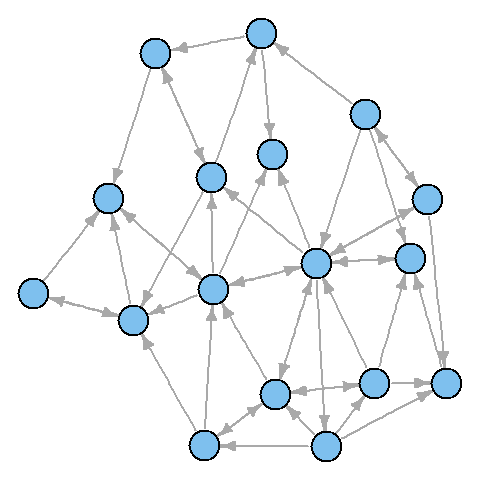
Now that there is a igraph network, you can make the first attempt to build it.

It turned out not too beautiful. Let's start improving the picture by removing the cycles in the graph.
You can note that you could use
Let's also reduce the size of the arrows and remove the labels (by setting them to
In part 2: fonts and colors in graphs R.
Introduction: Network Visualization
The main thing when designing a network visualization is the goal to be achieved. What structural properties would we like to highlight?
Network maps are by no means the only graph visualization tool - in some cases, other formats for representing networks are preferable, even simple graphs of key properties.
In maps of networks, as well as in other visualization formats, there are several key settings that affect the final result. The main ones are color, size, shape and relative position.
')
Modern graph views are optimized based on performance requirements and aesthetic considerations. In particular, it is necessary to minimize the overlap and intersection of the edges, to establish the same length of edges in the graph.
Data format, size and preparation
In this guide, we will mainly work with two small datasets. Both contain information about the media. One contains a network of hyperlinks and mentions in news resources. Another is a network of links between objects and mass media consumers. Although there is little data in the examples, many of the ideas from the generated visualizations can be extended to medium and large networks. For the same reason, we will rarely use visual tools, for example, the shape of vertex symbols: they are almost impossible to distinguish in large graphs. Moreover, when displaying very large networks, you can even hide edges, since you need to focus on identifying and displaying groups of vertices. Generally speaking, the size of networks that can be visualized with R is limited only by the amount of RAM in your machine. But it should be emphasized that in many cases the visualization of large networks in the form of a giant pom-pom is far less useful than graphs with the key properties of the graph.
This guide uses several key packages that must be installed before proceeding. Some more libraries will be mentioned, but they are optional and can be skipped. The following main libraries will be used - igraph (supported by Gabor Zardi and Tamas Nepush ), sna , network (supported by Carter Butts and the Statnet team ) and ndtv (supported by Sky Bender de Moll ).
install.packages("igraph") install.packages("network") install.packages("sna") install.packages("ndtv") Data Set 1: Edge List
The first data set to work with consists of two files: “Media-Example-NODES.csv” and “Media-Example-EDGES.csv” (you can download it here ).
nodes <- read.csv("Dataset1-Media-Example-NODES.csv", header=T, as.is=T) links <- read.csv("Dataset1-Media-Example-EDGES.csv", header=T, as.is=T) Examine the data:
head(nodes) head(links) nrow(nodes); length(unique(nodes$id)) nrow(links); nrow(unique(links[,c("from", "to")])) Please note that there are more edges than unique “from” - “to” combinations. This means that there are cases in the data when there is more than one connection between two vertices. We will roll all the edges of the same type between two nodes, summing their weights using the
aggregate() function on "from", "to" and "type": links <- aggregate(links[,3], links[,-3], sum) links <- links[order(links$from, links$to),] colnames(links)[4] <- "weight" rownames(links) <- NULL Data Set 2: Matrix
nodes2 <- read.csv("Dataset2-Media-User-Example-NODES.csv", header=T, as.is=T) links2 <- read.csv("Dataset2-Media-User-Example-EDGES.csv", header=T, row.names=1) Examine the data:
head(nodes2) head(links2) You can verify that the links2 is the mating matrix for a two-way network:
links2 <- as.matrix(links2) dim(links2) dim(nodes2) Network visualization: first steps with igraph
Let's start by turning the source data into a igraph network. To do this, we use the function igraph graph.data.frame, which takes as input two data blocks: d and vertices.
- d describes the edges of the network. The first two columns contain the identifiers of the starting and ending vertices for each edge. The following columns are the parameters of the edge (weight, type, label, other).
- vertices starts with a vertex identifier column. All the following columns are interpreted as vertex parameters.
library(igraph) net <- graph.data.frame(links, nodes, directed=T) net ## IGRAPH DNW- 17 49 -- ## + attr: name (v/c), media (v/c), media.type (v/n), type.label ## (v/c), audience.size (v/n), type (e/c), weight (e/n) The description of the igraph object begins with four letters:
- D or U - for directed or undirected graph, respectively.
- N - for a named graph (where nodes have an attribute
name). - W for a weighted graph (where links have a
weightattribute). - B - for a two-sided graph (where nodes have a
typeattribute).
The next two numbers (17 49) indicate the number of vertices and edges in the graph. The description also lists the properties of vertices and edges, for example:
(g/c)- string property at graph level(v/c)- vertex-level string property(e/n)- property-number at edge level
It is also easy to access vertices, edges and their attributes:
E(net) # "net" V(net) # "net" E(net)$type # "type" V(net)$media # "media" # : net[1,] net[5,7] Now that there is a igraph network, you can make the first attempt to build it.
plot(net) # ! It turned out not too beautiful. Let's start improving the picture by removing the cycles in the graph.
net <- simplify(net, remove.multiple = F, remove.loops = T) You can note that you could use
simplify to collapse several edges into one by summing their weights with a command like simplify(net, edge.attr.comb=list(Weight="sum","ignore")) . The problem is that the combination does not take into account the type of the edge (in our data, “hyperlinks” - links and “mentions” - references).Let's also reduce the size of the arrows and remove the labels (by setting them to
NA ): plot(net, edge.arrow.size=.4,vertex.label=NA) In part 2: fonts and colors in graphs R.
Source: https://habr.com/ru/post/262079/
All Articles