Statistical analysis of association rules in survey results
In the previous part of the article, the method of searching for associative rules in European social research data was considered. This part is about statistical analysis of the rules obtained. The key point is that classical statistical methods, for example, the chi-square agreement criterion, have no reason to be used for the survey results. But for what reasons? And how to test hypotheses? This will be discussed in this publication.

')
First briefly about survey methods. One of the characteristics of a qualitative survey is the representativeness of the sample. Respondents selected from the general population in a random, equally probable way and without returns determine simple random sampling. For a number of reasons, it is very difficult to obtain a representative simple random sample. Usually, the population is divided into strata for representativeness and clusters are allocated in each stratum to reduce the cost of the survey. In addition, in order to obtain an unbiased estimate of known population indicators (gender, age groups, ...), weights are attributed to respondents who participated in the study. Details can be found in the article A. Churikova [1].
The sample obtained using stratification, clustering and weighting ceases to be a simple random one. For variables of such a sample, the iid principles required in classical statistical tests are violated. In particular, clustering the sample increases the statistical error of the results due to the intraclass correlation of the observed values.
Another example of the difference from the “usual” formulas is finding the variance for the sample mean. Let x be a numerical or logical polling variable with a weight w . Then

Therefore, the ratio of the functions u / v is lianerised with the help of a Taylor series (limited to decomposition to terms of the first order) and a variance is found for each member of this series. This method of estimating the variance of the sample mean is not the only one; there are other ways. Details, formulas and examples can be found in Chapter 3, books [2].
Fortunately, in R there is a survey package that allows for statistical analysis of data obtained by respondents. The author of this package T. Lumley has written a detailed user manual, published in the form of a book [3]. For those who worked with the results of polls in other software - SAS, Stata, SUDAAN, article [4] is available. In addition, on the support web page of the book [2] , for most of the examples of this edition, the code is published in several programming languages, in particular for R.
In the ESS data for each country there is information about strata (stratify), clusters (psu - primary sample unit) and probabilities of respondents (prob). Weight is usually inversely proportional to probability. So, for Russia, the strata are federal districts, clusters are a number of cities and districts in these districts. Details and examples about the design of surveys in the ESS are given in this pdf taken from the project site.
Formulation of the problem.
In the previous part of the article the following results were obtained for one of the found rules:

Let me remind you, here Antecedent - the left part of the rule X -> Y , means that the respondents
- completely agree with the statement that for most people in the country, life becomes worse rather than better
and
- do not personify yourself with a person for whom it is important to be rich, to have a lot of money and expensive things.
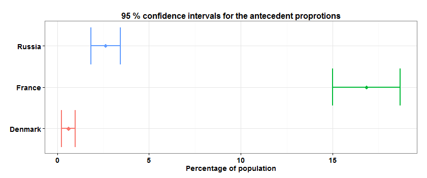
It is necessary to find confidence intervals for the shares of X in all three countries and to show that the result of supporting X in France is significantly different from the support of X in Denmark and Russia.
Data preparation.
In the resulting database ask the design of the study
The solution of the problem.
The svymean () function of the survey package finds not only the sample mean, but, in particular, its standard deviation, taking into account the study design. Then the confidence interval for the fraction p equal to the support of X for each country separately can be found as .
.
I will add that binomial methods for estimating confidence intervals of shares are also available in the survey package - the svyciprop () function.
To confirm the significance of the differences in the X support shares in the countries under consideration, we construct a logistic regression of the form

The coefficients of this linear model mean exactly the same as in the "usual" logistic regression. I.e

The results of this model show that the coefficients B_1 and B_2 are significantly different from zero. That is, the share of support X in France is statistically significantly different from the corresponding shares in Denmark and Russia.

And finally, we reject the null hypothesis that both model coefficients, B_1 and B_2 , are simultaneously equal to zero.
Since the X support values in the three countries examined are very different, the null hypotheses for logistic regression coefficients could be rejected without using information about the design of the survey. I did not set out to demonstrate an example in which the hypothesis was accepted or rejected, with some fixed level of error, depending on whether we use the data from the survey design or not.
However, such situations are quite likely. Consider example 6.8 from the book [2]: using the NCS-R Data, whose calculations can be fully reproduced using the R code ( pdf ) from the web page of this book. .
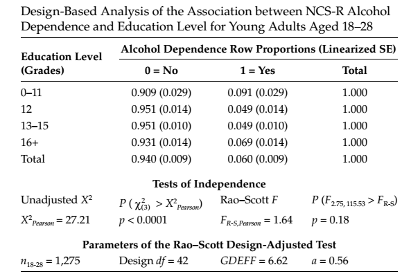
In this example, the null hypothesis of the independence of the variables "diagnosed alcohol dependence" and "level of education" among US citizens aged 18-28 years is tested. The standard criterion X ^ 2 rejects this hypothesis with an error probability of less than 1%, that is, we can confidently say that there is a relationship between these variables in the specified population. Whereas the chi-square test, adjusted by Rao-Scott for the study design, determines the magnitude of the erroneous deviation of the null hypothesis by more than 10%. It turns out that it is no longer possible to reject the null hypothesis at the 5% level.
Therefore, in the general case, a statistical analysis of the results of surveys is desirable to conduct with regard to the design of research.
In conclusion, I note that recently, structural equation modeling has been used to analyze cross-country results. One reason for this is that the stratification and clustering of the sample is usually done at the country level (in the ESS that way), and not in the general population. But about this sometime later, until I mention the collection of articles [5].
Literature:
[1] A. Churikov. Random and non-random samples in sociological studies, well. Social Reality, 4, 2007, pp. 89-109.
[2] Heeringa SG, West BT, Berglund PA Applied Survey Data Analysis, CRC Press, 2010.
[3] Lumley T. Complex Surveys: A Guide to Analysis Using R, Wiley, 2010.
[4] Damico A. Transitioning to R: Replicating SAS, Stata, and SUDAAN Analysis Techniques in Health Policy Data, The R Journal Vol. 1/2, December 2009.
[5] Cross-Cultural Analysis: Methods and Applications (edited by Davidov E., Schmidt P., Billiet J.), Routledge, 2011.
')
First briefly about survey methods. One of the characteristics of a qualitative survey is the representativeness of the sample. Respondents selected from the general population in a random, equally probable way and without returns determine simple random sampling. For a number of reasons, it is very difficult to obtain a representative simple random sample. Usually, the population is divided into strata for representativeness and clusters are allocated in each stratum to reduce the cost of the survey. In addition, in order to obtain an unbiased estimate of known population indicators (gender, age groups, ...), weights are attributed to respondents who participated in the study. Details can be found in the article A. Churikova [1].
The sample obtained using stratification, clustering and weighting ceases to be a simple random one. For variables of such a sample, the iid principles required in classical statistical tests are violated. In particular, clustering the sample increases the statistical error of the results due to the intraclass correlation of the observed values.
Another example of the difference from the “usual” formulas is finding the variance for the sample mean. Let x be a numerical or logical polling variable with a weight w . Then
Therefore, the ratio of the functions u / v is lianerised with the help of a Taylor series (limited to decomposition to terms of the first order) and a variance is found for each member of this series. This method of estimating the variance of the sample mean is not the only one; there are other ways. Details, formulas and examples can be found in Chapter 3, books [2].
Fortunately, in R there is a survey package that allows for statistical analysis of data obtained by respondents. The author of this package T. Lumley has written a detailed user manual, published in the form of a book [3]. For those who worked with the results of polls in other software - SAS, Stata, SUDAAN, article [4] is available. In addition, on the support web page of the book [2] , for most of the examples of this edition, the code is published in several programming languages, in particular for R.
In the ESS data for each country there is information about strata (stratify), clusters (psu - primary sample unit) and probabilities of respondents (prob). Weight is usually inversely proportional to probability. So, for Russia, the strata are federal districts, clusters are a number of cities and districts in these districts. Details and examples about the design of surveys in the ESS are given in this pdf taken from the project site.
Formulation of the problem.
In the previous part of the article the following results were obtained for one of the found rules:
Let me remind you, here Antecedent - the left part of the rule X -> Y , means that the respondents
- completely agree with the statement that for most people in the country, life becomes worse rather than better
and
- do not personify yourself with a person for whom it is important to be rich, to have a lot of money and expensive things.
It is necessary to find confidence intervals for the shares of X in all three countries and to show that the result of supporting X in France is significantly different from the support of X in Denmark and Russia.
Data preparation.
Download ESS 6 wave data (version 2.1) and survey design information to R
The data is uploaded to the public, but registration is required to download them. After authorization, download stata data from here to the working directory R.
# Danish survey design data
# French survey design data
# Russian survey design data
library(foreign) # to read data library(data.table) # to manipulate data srv.data <- read.dta("ESS6e02_1.dta") srv.variables <- data.table(name = names(srv.data), title = attr(srv.data, "var.labels")) srv.data <- data.table(srv.data) setkey(srv.data, cntry) setkey(srv.variables, name) # Danish survey design data
dk.dt <- data.table(read.dta("ESS6_DK_SDDF.dta")) dk.dt <- dk.dt[cntry!="NA",] # sic! this base contains extra records with NA data dk.dt[,stratify:="dk"] # dk sample is simple random sample dk.dt[,psu:=seq(3300,length.out = nrow(dk.dt))] #to avoid duplication with psu numbers of the fr data # French survey design data
fr.dt <- data.table(read.dta("ESS6_FR_SDDF.dta")) # Russian survey design data
ru.dt <- data.table(read.dta("ESS6_RU_SDDF.dta")) We form the required database and add a variable to it with the support of approval X
countries.set <- c("FR", "DK", "RU") cntries.srv.data <- srv.data[J(countries.set)] setkey(cntries.srv.data, cntry, idno) # idno is unique respondent's ID inside cntry cntries.dt <- rbind(dk.dt, fr.dt, ru.dt) setkey(cntries.dt, cntry,idno) cntries.srv.data <- cntries.srv.data[cntries.dt] # merge the databases cntries.srv.data[,weight:=dweight*pweight] # weight is defined as design weight adjusted on the countries population sizes # add antecedent (denoted as lhs) statement to the cntries.srv.data lhs.rule.adding<-function(lhs){ statements <- unlist(strsplit(lhs, " & ")) statements <- lapply(statements, function(l) unlist(strsplit(l,"="))) statements <- lapply( statements, function(l) c(question.name=srv.variables[title==l[1], name], answer=l[2]) ) conditions <- sapply( statements, function(l) paste("ifelse(is.na(", l[1], "), 0, ", l[1], " == '", l[2], "')", sep="") ) conditions <- paste(conditions, collapse = " & ") add.lhs.to.base <- paste("cntries.srv.data[,x:=", conditions,"]",sep="") eval(parse(text=add.lhs.to.base)) cntries.srv.data[,x:=as.numeric(x)] return(T) } lhs.rule.adding("For most people in country life is getting worse=Agree strongly & Important to be rich, have money and expensive things=Not like me") cntries.srv.data[,cntry:=factor(cntry, levels = countries.set)] In the resulting database ask the design of the study
library(survey) design.cntries.data <- svydesign(ids = ~psu, strata = ~stratify, weights = ~weight, data = cntries.srv.data) The solution of the problem.
The svymean () function of the survey package finds not only the sample mean, but, in particular, its standard deviation, taking into account the study design. Then the confidence interval for the fraction p equal to the support of X for each country separately can be found as
.R code for finding confidence intervals and plotting
X.supp.confint <- sapply(countries.set, function(country) { design.dt<-subset(design.cntries.data, cntry==country) w.mean<-svymean(~x, design.dt) c(w.mean[1],confint(w.mean,df = degf(design.dt))[1,]) }) X.supp.confint <- data.table(t(X.supp.confint)*100, country=c("France", "Denmark", "Russia")) setnames(X.supp.confint, 1:3, c("mean","lower","upper")) library(ggplot2) limits <- aes(xmax = upper, xmin=lower) p <- ggplot(X.supp.confint, aes(y=country, x=mean, colour=country)) + geom_point(size=4, shape=18) + geom_errorbarh(limits, width=0.2, lwd=1.0) p <- p + ggtitle("95 % confidence intervals for the antecedent proprotions") + xlab("Percentage of population") p + theme_bw() + theme(plot.title=element_text( face="bold", size=16), axis.text.y = element_text( face="bold", size=14), axis.text.x = element_text( face="bold", size=14), axis.title.x=element_text( face="bold", size=14), axis.title.y=element_blank(), legend.position="none") I will add that binomial methods for estimating confidence intervals of shares are also available in the survey package - the svyciprop () function.
To confirm the significance of the differences in the X support shares in the countries under consideration, we construct a logistic regression of the form
model <- svyglm(x~ cntry, design = design.cntries.data, family=quasibinomial) The coefficients of this linear model mean exactly the same as in the "usual" logistic regression. I.e
sapply(c(coef(model)[1], sum(coef(model)[c(1,2)]), sum(coef(model)[c(1,3)])), function(b) exp(b)/(1+exp(b)))*100 The results of this model show that the coefficients B_1 and B_2 are significantly different from zero. That is, the share of support X in France is statistically significantly different from the corresponding shares in Denmark and Russia.
library(DT); datatable(round(coef(summary(model)),4)) And finally, we reject the null hypothesis that both model coefficients, B_1 and B_2 , are simultaneously equal to zero.
regTermTest(model, ~cntry, method = "LRT") Working (Rao-Scott+F) LRT for cntry in svyglm(formula = x ~ cntry, design = design.cntries.data, family = quasibinomial) Working 2logLR = 379.0228 p= < 2.22e-16 (scale factors: 1.2 0.8 ); denominator df= 2088 Since the X support values in the three countries examined are very different, the null hypotheses for logistic regression coefficients could be rejected without using information about the design of the survey. I did not set out to demonstrate an example in which the hypothesis was accepted or rejected, with some fixed level of error, depending on whether we use the data from the survey design or not.
However, such situations are quite likely. Consider example 6.8 from the book [2]: using the NCS-R Data, whose calculations can be fully reproduced using the R code ( pdf ) from the web page of this book. .
In this example, the null hypothesis of the independence of the variables "diagnosed alcohol dependence" and "level of education" among US citizens aged 18-28 years is tested. The standard criterion X ^ 2 rejects this hypothesis with an error probability of less than 1%, that is, we can confidently say that there is a relationship between these variables in the specified population. Whereas the chi-square test, adjusted by Rao-Scott for the study design, determines the magnitude of the erroneous deviation of the null hypothesis by more than 10%. It turns out that it is no longer possible to reject the null hypothesis at the 5% level.
Therefore, in the general case, a statistical analysis of the results of surveys is desirable to conduct with regard to the design of research.
In conclusion, I note that recently, structural equation modeling has been used to analyze cross-country results. One reason for this is that the stratification and clustering of the sample is usually done at the country level (in the ESS that way), and not in the general population. But about this sometime later, until I mention the collection of articles [5].
Literature:
[1] A. Churikov. Random and non-random samples in sociological studies, well. Social Reality, 4, 2007, pp. 89-109.
[2] Heeringa SG, West BT, Berglund PA Applied Survey Data Analysis, CRC Press, 2010.
[3] Lumley T. Complex Surveys: A Guide to Analysis Using R, Wiley, 2010.
[4] Damico A. Transitioning to R: Replicating SAS, Stata, and SUDAAN Analysis Techniques in Health Policy Data, The R Journal Vol. 1/2, December 2009.
[5] Cross-Cultural Analysis: Methods and Applications (edited by Davidov E., Schmidt P., Billiet J.), Routledge, 2011.
Source: https://habr.com/ru/post/262005/
All Articles