^{Captain Nemo at the helm "Nautilus"}

Indexes are one of the most powerful tools in relational databases. We use them when we need to quickly find some values, when we merge databases, when we need to speed up the work of SQL statements, etc. But what are the indices? And how do they help speed up the search in the database? To answer these questions, I examined the PostgreSQL source code, tracking how an index is searched for a simple string value. I expected to find complex algorithms and efficient data structures. And found.

Here I will talk about how the indexes are arranged and how they work. However, I did not expect that they are based on informatics. In the understanding of the underpotted indexes, comments in the code also helped, explaining not only how Postgres works, but why it works that way.

Search for sequences

The sequence search algorithm in Postgres shows oddities: for some reason, it looks at all the values ​​in the table. In my last post, I used this simple SQL statement to look up the meaning of “Captain Nemo”:
')


Postgres sparsil, analyzed and planned the request. Then ExecSeqScan (a C-language built-in function that implements the SEQSCAN sequence search) quickly found the desired value:



But then, for an inexplicable reason, Postgres continued to scan the entire database, comparing each value with the desired one, although it was already found!



If the table contained millions of values, the search would take a lot of time. Of course, this can be avoided by removing the sort and rewriting the query so that it stops at the first match found. But the problem is deeper, and it lies in the inefficiency of the search engine itself in Postgres. Using the search sequence to compare each value in the table - the process is slow, inefficient and dependent on the order of the records. There must be another way!

The solution is simple: you need to create an index.

Create index

Make it simple, just run the command:


Ruby developers would prefer to use the add_index migration using ActiveRecord, in which the same CREATE INDEX command would be executed. Normally, when we restart select, Postgres creates a scheduling tree. But in this case it will be slightly different:



Notice that INDEXSCAN is used at the bottom instead of SEQSCAN. INDEXSCAN will not scan the entire database, unlike SEQSCAN. Instead, it uses the newly created index to quickly and efficiently find the desired entry.

Creating an index solves a performance problem, but does not provide answers to a number of questions:

• What exactly is an index in Postgres?
• How exactly does it look like, what is its structure?
• How does the index speed up the search?

Let's answer these questions by studying the source code in C.

What is an index in Postgres

Let's start with the documentation for the CREATE INDEX command :



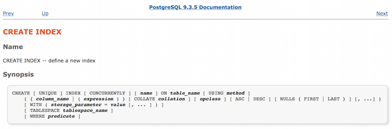
All parameters that can be used to create an index are displayed here. Pay attention to the parameter USING method: it describes what kind of index we need. The same page contains information about the method, the argument of the USING keyword:



It turns out that four different types of indexes are implemented in Postgres. They can be used for different types of data or depending on the situation. Since we did not define the USING parameter, the default index_users_on_name is an index of the form “btree” (B-Tree).

What is B-Tree and where can I find information about it? To do this, examine the appropriate Postgres source file:



This is what it says about in the README:



By the way, the README itself is a 12-page document. That is, we have access to not only useful comments in the C code, but also all the necessary information about the theory and concrete implementation of the database server. Reading and parsing code in opensource projects is often a daunting task, but not in Postgres. The developers have tried to facilitate our process of understanding the device of their offspring.

Please note that in the very first sentence there is a link to a scientific publication that explains what B-Tree is (and therefore, how the indexes work in Postgres): Efficient Locking for Leopards and Yao (Yao).

What is B-Tree

The article describes the improvement made by the authors in the B-Tree algorithm in 1981. We will talk about this later. The algorithm itself was developed in 1972, as is the example of a simple B-Tree:



The name is short for English. “Balanced tree”. The algorithm allows you to speed up the search operation. For example, we need to find the value 53. Let's start with the root node containing the value 40:



It is compared with the desired value. Since 53> 40, then we follow the right branch of the tree. And if we were looking for, for example, the value 29, we would go along the left branch, because 29 <40. Following the right branch, we find ourselves in a child node containing two values:



This time we compare 53 with the values ​​47 and 62: 47 <53 <62. Notice that the values ​​inside the nodes are sorted. Since the desired value is less than one and more than the other, then we follow the central branch and get to the child node containing three values:



We compare with the list of sorted values ​​(51 <53 <56), go to the second of the four branches and finally get to the child node with the desired value:



Due to what this algorithm speeds up the search:

1. Values ​​(keys) within each node are sorted.
2. The algorithm is balanced : the keys are evenly distributed over the nodes, which allows minimizing the number of transitions. Each branch leads to a child node that contains approximately the same number of keys as all other child nodes.

What does an index in Postgres look like

Lehman and Yao drew their diagram over 30 years ago. What does it have to do with modern Postgres? It turns out that the index_users_on_name we created is very similar to this very diagram. When executing the CREATE INDEX command, Postgres stores all values ​​from the user table as keys of the B-Tree tree. This is the index node:



Each entry in the index consists of a structure in the C language, called IndexTupleData, and also contains a value and a bitmap. The latter is used to save space, it records information about whether index attributes in the key accept NULL values. The values ​​themselves follow the bitmap in the index.

Here is the structure of IndexTupleData:



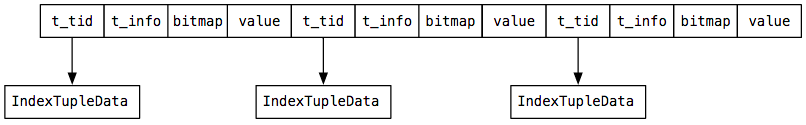
t_tid : this is a pointer to some other index or database entry. Note that this is not a pointer to the physical memory from the C language. Here is the data by which Postgres searches for the associated memory pages.

t_info : contains information about the index elements. For example, how many values ​​are stored in it, are they equal to NULL, etc.

For better understanding, consider several entries from index_users_on_name :



Here, instead of value, some names from the database are inserted. The node from the top tree contains the keys “Dr. Edna Kunde ”and“ Julius Powlowski ”, and the lower node -“ Julius Powlowski ”and“ Juston Quitzon ”. Unlike the Lehmann and Yao diagrams, Postgres repeats the parent keys in each child node. For example, “Julius Powlowski” is the key in the top tree and in the child node. The t_tid pointer refers to Julius in the top node to the same name in the bottom node. If you want to learn more about storing key values ​​in B-Tree nodes, refer to the file itup.h:

Search for a B-Tree node containing our value

Let's go back to our original SELECT statement:

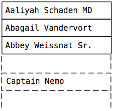
How exactly is Postgres searching for the value of “Captain Nemo” in the index_users_on_name index? Why does using an index allow you to search faster compared to finding a sequence? Let's take a look at some of the names stored in our index:



This is the root node at index_users_on_name. I just unfolded the tree so that the names fit entirely. Here are four names and one null value. Postgres automatically created this root node as soon as the index itself was created. Note that with the exception of NULL, which indicates the beginning of the index, the other four names are in alphabetical order.

As you remember, B-Tree is a balanced tree. Therefore, in this example, the tree has five child nodes:

• Alphabetical names for “Dr. Edna Kunde ”
• The names between “Dr. Edna Kunde ”and“ Julius Powlowski ”
• Names between “Julius Powlowski” and “Monte Nicolas”
  …etc.

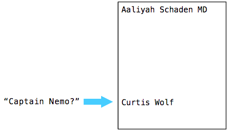
As we are looking for “Captain Nemo”, Postgres follows the first branch to the right (when alphabetically sorting, the desired value goes to “Dr. Edna Kunde”):



As you can see from the illustration, further Postgres finds the node with the desired value. For the test, I added 1000 names to the table. This right knot contained 240 of them. So the tree significantly accelerated the search process, since the remaining 760 values ​​were left out.

If you want to learn more about the search algorithm for the desired node in B-Tree, refer to the comments to the _bt_search function.

Finding our value inside the node

So Postgres has moved to a node containing 240 names, among which he needs to find the value “Captain Nemo”.



For this purpose, it is not a search sequence, but a binary search algorithm. First, the system compares the key that is in the middle of the list (position 50%):



The desired value is in alphabetical order after “Breana Witting”, so Postgres jumps to the key in the 75% position (three-fourths of the list):



This time our value should be higher. Then Postgres jumps some value higher. In my case, the system took eight times to jump through the list of keys in the node, until it finally found the desired value:



You can read more about the algorithm for searching the values ​​inside the node in the comments to the _bt_binsrch function:

Other interesting things

If you have a desire, then a certain amount of theory about B-Tree trees can be gleaned from the scientific work of Efficient Locking for Concurrent Operations on B-Trees .

Adding keys to B-Tree . The procedure for introducing new keys into the tree is performed using a very interesting algorithm. Typically, the key is written to the node in accordance with the accepted sorting. But what to do if there is no free space in the node? In this case, Postgres divides the node into two smaller ones and inserts a key into one of them. It also adds a key from the “split point” and a pointer to the new child node to the parent node. Of course, the parent node also has to be split in order to insert this key, as a result, the procedure of adding a single key to the tree turns into a complex recursive operation.

Deleting keys from B-Tree . Also a rather curious procedure. When deleting a key from some node, Postgres, if possible, merges its child nodes. This can also be a recursive operation.

B-Link-Tree trees . In fact, Lehmann and Yao’s work describes an innovation invented by them related to parallelism and blocking, when one tree is used by several threads. Postgres code and its algorithms must support multi-threading, because several clients can access (or modify it) a single index simultaneously. If you add a pointer from each node to the next child node ("right arrow"), then one thread can search the tree, while the other will split the node without blocking the entire index:

Do not be afraid to explore

Perhaps you know all about how to use Postgres, but do you know how it is arranged inside, what is “under the hood”? The study of computer science, in addition to working on current projects, is not fun, but part of the development process of the developer. Year by year, our software tools are becoming more complex, multifaceted, better, making it easier for us to create websites and applications. But we must not forget that the basis of all this is the science of computer science. We, like the entire community of Postgres opensource developers, stand on the shoulders of our predecessors, such as Lehman and Yao. Therefore, do not blindly trust the tools that you use every day, study their device. This will help you to achieve a higher professional level, you can find information and solutions for yourself that you had never known before.