Magic of tensor algebra: Part 4 - Dynamics of a point in a tensor statement

Content

Introduction

So, the time has come to put into practice everything that we have been reasoning about theoretically for so long. This note will mainly use material from the previous article , which contains links to previous publications on tensor topics.

And we will deal with mechanics. It was the solution of the problems of mechanics that prompted me to deal with tensor calculus. And we will talk about the Lagrange equations of the 2 kind, which are used to analyze the movement of complex mechanical systems. These equations have the form well known to most experts in this field.
')

$\ frac {d} {dt} \ left (\ frac {\ partial T} {\ partial \ dot {q} ^ i} \ right) - \ frac {\ partial T} {\ partial q ^ i} = Q_i \ quad i = \ overline {1, s}$

where s is the number of degrees of freedom of the mechanical system; $q ^ i$ - generalized coordinate; $T = T \ left (\ vec {q}, \, \ dot {\ vec {q}} \ right)$ - the kinetic energy of the mechanical system; $Q ^ i$ - generalized force.

Those who came across these equations probably noticed that after performing a three-fold differentiation of the kinetic energy, expressions are obtained that are represented by a linear combination of the second derivatives of the generalized coordinates and a linear combination of the products of their first derivatives. And this, at least for me, suggested that kinetic energy can be differentiated once in a general form, and then simply make up the equations of motion using the obtained expressions of a general form. Only now attempts to do it yourself did not lead me to success.

Nevertheless, this can be done if we rely on tensor calculus, in general, without resorting to the differentiation of the kinetic energy (although this approach is also possible). And we will do it in this article, though so far only for a point, and at the same time we will solve some not too complicated task, illustrating the effectiveness of the considered approach.

Well, let's start!

1. Kinematics of a material point in arbitrary coordinates

The traditional way of presenting mechanics is the vector method of defining the motion of a point.

Fig. 1. Vector way to set the point motion

With this method of specifying the motion, the position of a point in space is determined by the radius vector, released from some point O , by which the reference body is meant. This radius vector is a function of time.

$\ vec {r} = \ vec {r} \, (t) \ quad (1)$

If function (1) is given, then they say that the law of motion of a point is given . Knowing the law of motion of a point, you can get its speed and acceleration.

$\ vec {v} = \ frac {d \ vec {r}} {dt}, \ quad \ vec {a} = \ frac {d \ vec {v}} {dt} = \ frac {d ^ 2 \ vec {r}} {dt ^ 2} \ quad (2)$

Radius vector, speed and acceleration are vectors, which means we will consider them as rank (1.0) tensors. In addition, we will not use the Cartesian coordinate system. We will use curvilinear coordinates

$q ^ i = q ^ i \, (t) \ quad i = \ overline {1, s} \ quad (3)$

Where $q ^ i$ - a set of independent parameters that uniquely characterize the position of a point in space. And there will not necessarily be three of these parameters, there may be fewer, it all depends on how many degrees of freedom s the point in question has. Such coordinates in analytical mechanics are called generalized .

The determination of the number of degrees of freedom is formulated in two ways.

The number of degrees of freedom of a body is the difference between the number of dependent coordinates n , which uniquely determine the position of the body in space and the number of equations imposed on the body of bonds r

$s = n - r$

The number of coordinates that determine the position of a point in the space n = 3. If the motion of a point is not limited by constraints, then the number of degrees of freedom will also be equal to three.

If a point moves along a certain surface, then its movement is limited - the surface is a connection that imposes conditions on the Cartesian coordinates of the point. This condition is the equation of the surface on which the points move and is the equation of connection. The number of degrees of freedom of such a point is s = 2. The number of generalized coordinates will also be equal to two — these will be curvilinear coordinates measured along the surface.

If a point moves along a certain curve, then two connections are already superimposed on it — the curve in space is defined as the line of intersection of the two surfaces. The number of degrees of freedom of such a point is s = 1, and the generalized coordinate is one — the length of the arc that the point passed along the curve.

Thus, coordinates (3) automatically take into account the geometry of bonds imposed on a point, which in analytical mechanics allows us to exclude the reaction of bonds from the equations of motion.

Another definition of the number of degrees of freedom is

The number of degrees of freedom of the body - the number of independent parameters that uniquely determine the position of the body in space

also includes an idea of connections, but in a more veiled form.

We will call (3) the law of motion of a point. Knowing the law of motion, we obtain the velocity and acceleration vectors of the point. Differentiate in time the radius vector of a point

$\ vec {v} = \ frac {d \ vec {r}} {dt} = \ frac {\ partial \ vec {r}} {\ partial q ^ i} \, \ frac {dq ^ {\, i} } {dt} = \ frac {\ partial} {\ partial q ^ i} \ left (q ^ {\, j} \, \ vec {e} _j \ right) \ frac {dq ^ {\, i}} {dt} = \ frac {dq ^ {\, i}} {dt} \ vec {e} _i \ quad (4)$

I recall that in (4) the Einstein rule works and the right-hand side of the expression is summed over the silent indices i and j . Obviously, the partial derivative $\ frac {\ partial} {\ partial q ^ i} \ left (q ^ {\, j} \, \ vec {e} _j \ right) = \ vec {e} _i$ - coefficient of the component on which differentiation occurs. Expression (4) is the expansion of the velocity vector along a curvilinear basis, that is,

$\ dot {q} ^ {\, i} = \ frac {dq ^ {\, i}} {dt} \ quad (5)$

There are contravariant components of the velocity vector. Now, to get the acceleration vector, we differentiate by time (4)

$\ vec {a} = \ frac {d \ vec {v}} {dt} = \ frac {\ partial \ vec {v}} {\ partial q ^ {\, i}} \, \ dot {q} ^ {\, i} \ quad (5)$

We recall the definition of the covariant derivative from the previous article, we write the derivative of the velocity vector by the generalized coordinate (we look at the formula (33) from the previous publication

$\ frac {\ partial \ vec {v}} {\ partial q ^ {\, i}} = \ left (\ frac {\ partial \ dot {q} ^ {\, k}} {\ partial q ^ {\ , i}} + \ Gamma_ {ji} ^ {k} \ dot {q} ^ {\, j} \ right) \ vec {e} _k \ quad (6)$

Where $\ Gamma_ {ji} ^ {k}$ - symbols of Christoffel 2 kind

Substitute (6) into (5)

$\ vec {a} = \ left (\ frac {\ partial \ dot {q} ^ {\, k}} {\ partial q ^ {\, i}} + \ Gamma_ {ji} ^ {k} \ dot { q} ^ {\, j} \ right) \ dot {q} ^ {\, i} \, \ vec {e} _k = \ left (\ frac {\ partial \ dot {q} ^ {\, k} } {\ partial q ^ {\, i}} \, \ dot {q} ^ {\, i} + \ Gamma_ {ji} ^ {k} \, \ dot {q} ^ {\, j} \, \ dot {q} ^ {\, i} \ right) \, \ vec {e} _k \ quad (7)$

In equation (7), the first term in brackets

$\ frac {\ partial \ dot {q} ^ {\, k}} {\ partial q ^ {\, i}} \, \ dot {q} ^ {\, i} = \ ddot {q} ^ {\ , k} \ quad (8)$

the second derivative of the generalized time coordinate. In view of (8), we finally write the expression for the contravariant components of the point acceleration vector

$a ^ k = \ ddot {q} ^ {\, k} + \ Gamma_ {ji} ^ {k} \, \ dot {q} ^ {\, j} \, \ dot {q} ^ {\, i }, \ quad (9)$

2. Possible point movement

Let's start with the definition

Possible (or kinematically possible) is called such a movement of the point at which the superimposed on the connection point

This concept is basic in analytical mechanics. Consider the motion of a non-free point (Figure 2). Let the point move on the surface. Its coordinates can take only those values at which all points of the trajectory are located on a given surface. Such coordinates are called kinematically possible, they are interconnected by the surface equation. In this case, it is convenient to choose curvilinear coordinates. $q ^ {\, i}$ , which will take into account the fact that the point does not leave the surface (in this case we do not consider the conditions of release from communication). As we said above, such coordinates are called generalized.

Fig. 2. Possible movement of a non-free point.

We distort the generalized coordinates, that is, we add an infinitesimal function to the law of coordinate changes $\ delta q ^ {\, i}$ called the variation of the generalized coordinate

$\ tilde {q} ^ {\, i} = q ^ {\, i} + \ delta q ^ {\, i} \ quad (10)$

and calculate what movement the point will make

$\ delta \ vec {r} = \ frac {\ partial \ vec {r}} {\ partial q ^ {\, i}} \, \ delta q ^ {\, i} = \ vec {e} _ {\ , i} \, \ delta q ^ {\, i} \ quad (11)$

Vector $\ delta \ vec {r}$ and there is a possible movement of a point, and it is directed tangentially to the surface along which the point moves. As can be seen from (11), this vector is expanded on a local basis through contravariant components, which are variations of generalized coordinates $\ delta q ^ {\, i}$ . Due to the independence of generalized coordinates, their variations are also independent. This fact is useful to us in the future.

3. The general equation of point dynamics

Let us again refer to Figure 2. Let a nonfree point move under the action of active forces whose resultant is equal to $\ vec {F} ^ {\, a}$ . Since the point is not free, then reactions of bonds are attached to it, the resultant of which is equal to $\ vec {R}$ . By virtue of Newton's second law and the principle of independence of the action of forces, the vector equation

$m \, \ vec {a} = \ vec {F} ^ {\, a} + \ vec {R} \ quad (12)$

Multiply (12) scalarly by the possible displacement of a point (11)

$m \, \ vec {a} \ cdot \ delta \ vec {r} = \ vec {F} ^ {\, a} \ cdot \ delta \ vec {r} + \ vec {R} \ cdot \ delta \ vec {r} \ quad (12)$

Suppose the ideality imposed on the point of connections, which means that their reactions do not work on the possible movement of the point

$\ vec {R} \ cdot \ delta \ vec {r} = 0 \ quad (14)$

This, in principle, can always be allowed. With the presence of non-ideal bonds, their reactions under certain conditions can be translated into the category of active forces, which complicates the task, but it is not a fundamental difficulty. Analytical mechanics operates with this assumption, we will go the same way, putting the validity of (14) and coming to the equation

$m \, \ vec {a} \ cdot \ delta \ vec {r} = \ vec {F} ^ {\, a} \ cdot \ delta \ vec {r}$

Now, as proposed in relation (11), we expand the possible displacement through variations of generalized coordinates (implying summation over repeated indices)

$m \, (\ vec {a} \ cdot \ vec {e} _ {\, i}) \, \ delta q ^ {\, i} = (\ vec {F} ^ {\, a} \ cdot \ vec {e} _ {\, i}) \, \ delta q ^ {\, i} \ quad (15)$

In expression (15), the covariant projections of the point acceleration are on the left, and the covariant projections of the resultant active forces are on the right.

$m \, a _ {\, i} \, \ delta q ^ {\, i} = Q _ {\, i} \, \ delta q ^ {\, i} \ quad (16)$

In analytical mechanics $Q _ {\, i}$ called the generalized active force. Based on (15), we conclude that the generalized force is the covariant component of the resultant active forces.

Now we twist (9) with the metric tensor, substituting the result in (16)

$m \, g_ {ij} \, \ left (\ ddot {q} ^ {\, j} + \ Gamma_ {kl} ^ {\, j} \, \ dot {q} ^ {\, k} \, \ dot {q} ^ {\, l} \ right) \, \ delta q ^ {\, i} = Q _ {\, i} \, \ delta q ^ {\, i} \ quad (17)$

By virtue of the independence of variations of the generalized coordinates, the coefficients at them can be equated by obtaining s (by the number of generalized coordinates) equations

$m \, g_ {ij} \, \ left (\ ddot {q} ^ {\, j} + \ Gamma_ {kl} ^ {\, j} \, \ dot {q} ^ {\, k} \, \ dot {q} ^ {\, l} \ right) = Q _ {\, i} \ quad i = \ overline {1, s} \ quad (18)$

Does nothing remind you of the resulting equation (18)? This is very similar to the equations of motion, which are obtained after taking all the derivatives in the Lagrange equations of the second kind. Moreover, these are the Lagrange equations of the second kind - one can come to equations (18) by differentiating the kinetic energy, expressing it through the contravariant components of the velocity vector.

Similarly, in analytical mechanics, the Lagrange equations of the second kind are derived, based on an expression like (15), which in essence is the general dynamic equation written in generalized forces. In addition, equation (15) is invariant with respect to the coordinate transformation, because its left and right parts are scalar products of vectors. And the scalar product, as we remember, is an invariant with respect to the change of the basis.

Thus, we obtained the differential equations of the motion of a material point in generalized coordinates. Now apply them to solve the known problem.

4. The movement of a point under the action of a central force. Binet equation

Consider the movement of a heavy point in a plane, under the action of a force directed radially from the attracting / repelling center O. This task is a typical problem of a point moving in a central field and it has a simple analytical solution. Simple enough to try to solve it by applying equations (18) and test them

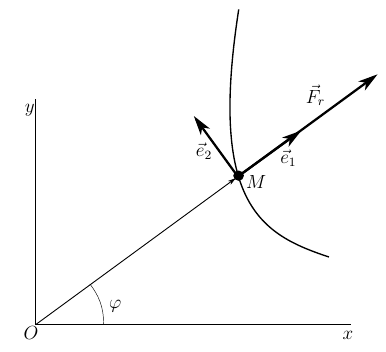
Fig. 3. Motion point in the central field.

The problem will be solved in polar coordinates

$q ^ 1 = r, \ quad q ^ 2 = \ varphi$

metrics for which is known (you can see here , but you can get it, but this is rather trivial)

$\ mathbf {g} = \ begin {bmatrix} 1 & amp & amp; 0 \\ 0 & amp; & amp; r ^ 2 \ end {bmatrix}$

For polar coordinates, it is easy to find Christoffel symbols of the 2 genus. Five of them are zero and only three are nonzero.

$\ Gamma_ {22} ^ 1 = -r$

$\ Gamma_ {12} ^ 2 = \ Gamma_ {21} ^ 2 = \ frac {1} {r}$

Using this data, you can write out the left side of equations (18)

$m \, g_ {11} \ left (\ ddot {q} ^ {\, 1} + \ Gamma_ {22} ^ 1 \, (\ dot {q} ^ {\, 2}) ^ 2 \ right) = m \ left (\ ddot {r} - r \, \ dot {\ varphi} ^ 2 \ right)$

$m \, g_ {21} \, \ left (\ ddot {q} ^ {\, 1} + 2 \, \ Gamma_ {12} ^ 2 \, \ dot {q} ^ 1 \ dot {q} ^ 2 \ right) + m \, g_ {22} \, \ left (\ ddot {q} ^ {\, 2} + 2 \, \ Gamma_ {12} ^ 2 \, \ dot {q} ^ 1 \ dot { q} ^ 2 \ right) = m \, r ^ 2 \, \ left (\ ddot {\ varphi} - \ frac {2} {r} \, \ dot {r} \, \ dot {\ varphi} \ right)$

Since the power $\ vec {F} _r$ radially directed, then at any point of the plane in question it is directed along the vector $\ vec {e} _1$ and perpendicular to the vector $\ vec {e} _1$ and based on the fact that the generalized force is determined by the scalar product of the resultant vector on the corresponding basis vector, we can write

$Q_1 = F_r, \ quad Q_2 = 0$

That is, get the equations of motion of a point

$\ ddot {r} - r \, \ dot {\ varphi} ^ 2 = \ frac {F_r} {m} \ quad (19)$

$r ^ 2 \, \ ddot {\ varphi} - 2 \, r \, \ dot {r} \, \ dot {\ varphi} = 0 \ quad (20)$

Equation (20) is easily integrated

$\ frac {d} {dt} \ left (r ^ 2 \, \ dot {\ varphi} \ right) = 0$

$r ^ 2 \, \ dot {\ varphi} = c \ quad (21)$

moreover, (21) expresses the constancy of the sector speed, which is characteristic of movement in the central field. From (21) we express the derivative with respect to the polar angle and substitute in (19)

$\ ddot {r} - \ frac {c ^ 2} {r ^ 3} = \ frac {F_r} {m} \ quad (22)$

In (22) we proceed from the differentiation in time to the derivative with respect to the polar angle

$\ dot {r} = \ frac {dr} {d \ varphi} \, \ dot {\ varphi} = \ frac {c} {r ^ 2} \, \ frac {dr} {d \ varphi} = -c \, \ frac {d} {d \ varphi} \ left (\ frac {1} {r} \ right) \ quad (23)$

$\ ddot {r} = \ frac {d \ dot {r}} {d \ varphi} \, \ dot {\ varphi} = \ frac {c} {r ^ 2} \, \ frac {d \ dot {r }} {d \ varphi} = - \ frac {c ^ 2} {r ^ 2} \, \ frac {d ^ 2} {d \ varphi ^ 2} \ left (\ frac {1} {r} \ right ) \ quad (24)$

Substitute (24) into (22)

$- \ frac {c ^ 2} {r ^ 2} \, \ frac {d ^ 2} {d \ varphi ^ 2} \ left (\ frac {1} {r} \ right) - \ frac {c ^ 2 } {r ^ 3} = \ frac {F_r} {m} \ quad (25)$

And, finally, multiplying both sides (25) by $- \ frac {r ^ 2} {c ^ 2}$ get

$\ frac {d ^ 2} {d \ varphi ^ 2} \ left (\ frac {1} {r} \ right) + \ frac {1} {r} = - \ frac {F_r \, r ^ 2} { m \, c ^ 2} \ quad (25)$

This equation is known as the Binet differential equation of a point in a central field. If the movement occurs under the action of Newton's, then

$F_r = - G \, \ frac {m \, M} {r ^ 2}$

And we get a general solution in the form

$\ frac {1} {r} = C_1 \ cos \ vaphi + C_2 \ sin \ varphi - \ frac {G \, M} {c ^ 2}$

which is the equation of conic sections (circles, ellipses, parabolas and hyperbolas) in polar coordinates

Conclusion

This article shows an approach to the use of tensor relations in relation to the dynamics of a material point, the movement of which can be described by arbitrary generalized coordinates. The equations obtained directly follow from the general principles of analytical mechanics and are equivalent to the Lagrange equations of the second kind.

This approach can be applied to the description of the motion of a mechanical system. But I will tell about it a bit later, but for now thanks to everyone who read this work for attention.

To be continued…

Source: https://habr.com/ru/post/261803/

All Articles