Hierarchical classification of sites in Python
Hi, Habr! As mentioned in the last article , an important part of our work is user segmentation. How do we do it? Our system sees users as unique cookies identifiers that we or our data providers assign to them. This id looks like this:
These numbers are keys in different tables, but the initial value is, first of all, the URL of the pages on which this cookie was downloaded, search queries, and sometimes some additional information that the provider gives - IP address, timestamp, customer information And so on. This data is rather heterogeneous, so the URL is the most valuable for segmentation. When creating a new segment, the analyst indicates a certain list of addresses, and if some cookie lights up on one of these pages, then it falls into the corresponding segment. It turns out that almost 90% of the working time of such analysts is spent on finding the right set of URLs - as a result of hard work with search engines, Yandex.Wordstat and other tools.
Having thus received more than a thousand segments, we realized that this process should be automated and simplified as much as possible, while being able to monitor the quality of the algorithms and provide analysts with a convenient interface for working with the new tool. Under the cut, I will tell you how we solve these problems.
So, as it was possible to understand from the introduction, in fact, it is not the users that need to be segmented, but the pages of Internet sites, - our analytic engine will automatically distribute users to the received segments.
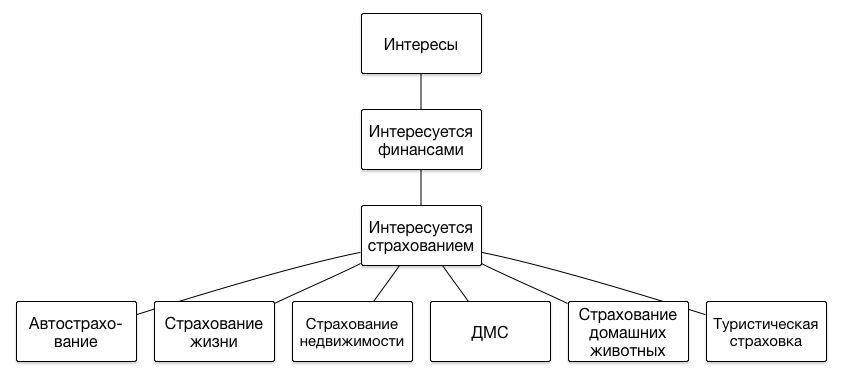
It is worth saying a few words about how the segments are represented in our DMP. The main feature of a set of segments is that their structure is hierarchical, that is, is a tree. We do not impose any restrictions on the depth of the hierarchy, since each next level allows us to more accurately describe the portrait of the user's interests. Here are examples of several branches of the hierarchy:
')
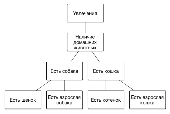
If a user has visited a site that tells how to feed puppies or train a cat to the tray, it is likely that he is the owner of this animal, and it makes sense to show him the corresponding advertisements - about the veterinary clinic or a new line of feed. And if, before that, he chose premium brands in his online store, then he could have relatively high incomes, and he could advertise more expensive services - a feline psychologist or a canine barber.
In general, having some kind of manual taxonomy of the subject of Internet pages, it was necessary to create a service that, given an input URL, would output a list of topics suitable for it. We solve the problem of determining the subject of a web page as a multi-class classification according to the “one against all” scheme, that is, each classifier of its taxonomy has its own classifier. Classifiers are recursively bypassed, starting from the root of the topic tree and further down along those branches that are identified as suitable at each current level.
The frontend classifier is a Flask application, which holds an object in memory. In essence, it deals only with data preparation, deserialization of objects of trained classifiers of the class sklearn.ensemble.RandomForestClassifier stored in mongoDB, execution of their predict_proba () methods and processing of results in accordance with the existing taxonomy. Taxonomy with queries and test samples, by the way, is also stored in mongoDB.
The application waits for POST requests by the URI of the form:
Obtaining, for example, a certain URL, the application downloads its body, extracts the text directly from there, and initiates a recursive taxonomy traversal from the root to the children. Recursion occurs only for those nodes of the tree for which at the current step the probability of a page being owned by this node exceeds the threshold specified in the config.
Data preparation includes one-time tokenization of the text, calculation of the frequency characteristics of words and a feature conversion for each classifier in accordance with the weights for the tokens selected at the stage of the selection selection (more on this later). This uses the “ bag of words ” model, that is, the relative position of words in the text is ignored.
The learning process performs the backend. When changes are made to the taxonomy or to the list of requests for a node, the texts of new pages are downloaded and tokenized, then the learning algorithm is launched for all topics at the same level as the changed one. All the “brothers” of the classifier are retrained along with the changed, because the training sample for the whole level is the same - the texts of the sites from the TOP-50 Bing search results, found from all nodes of the brothers and all their children. For each topic, positive examples are sites that match their needs and the needs of their children, all other pages are negative examples. The result is stored in the pandas.DataFrame object.
The resulting sets of tokens with labels are then randomly distributed to the training sample (70%), the sample for the feature selection (15%) and the test sample (15%) - it is stored in mongoDB.
The selection of the most informative tokens is carried out in the learning process using the dg metric, and this is how it is implemented:
And this is how it is called for a set of tokens:
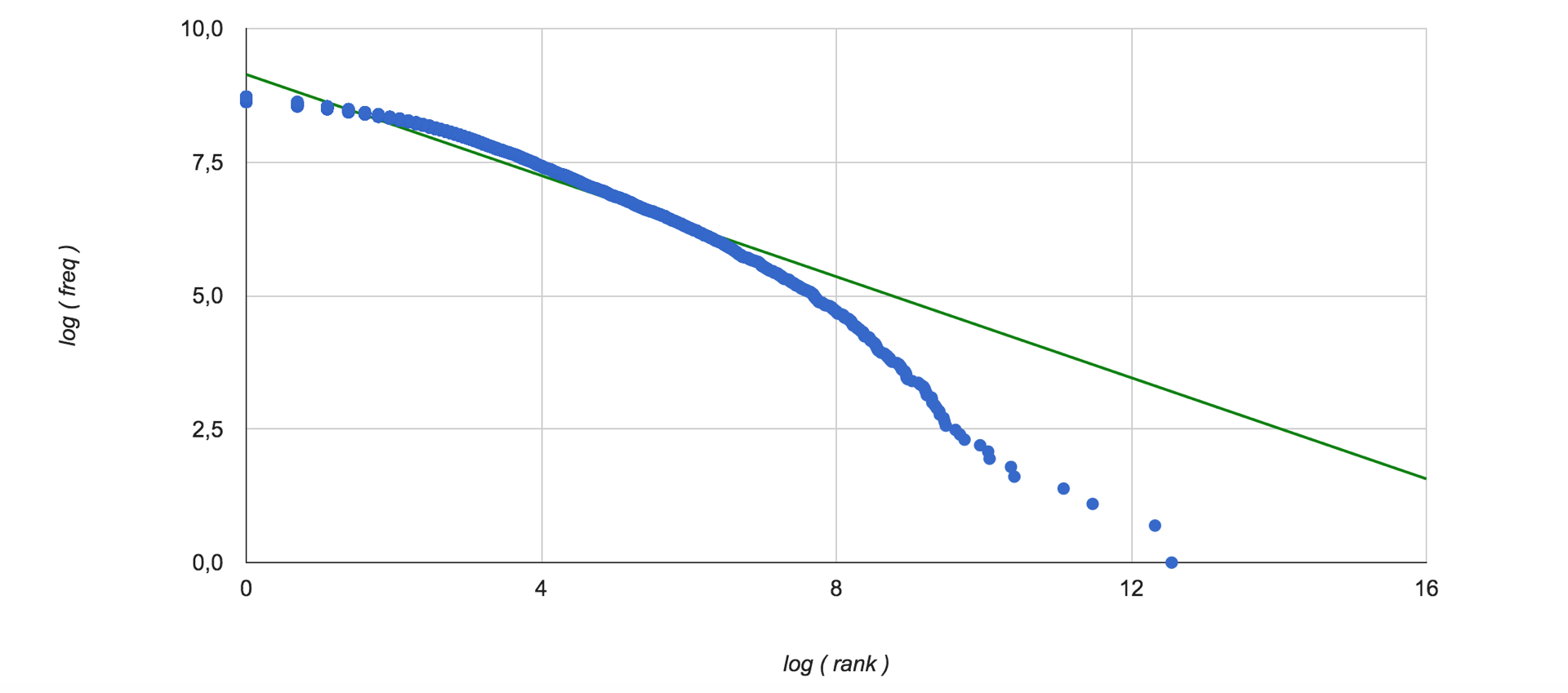
Thus, the significance of words is assessed from the point of view of all texts of the training set. Since the frequency characteristics of the occurrence of words in the collection are used, it is interesting to look at the Zipf distribution . Here it is (green color shows linear interpolation of data):
Further, for vectorization of classified texts, including in the learning process, the weight obtained in this way is multiplied by the frequency of the word in this text, and 5 words are selected with the highest value of this value for each topic at a given taxonomy level. These vectors are further concatenated, resulting in a vector of length 5 * m, where m is the number of nodes in the level. Now the data is ready for classification.
We wanted to be able to get one number to evaluate the work of the entire classifier as a whole. It is clear that it is easy to calculate the accuracy, completeness and F-measure for each individual taxonomy node, but when more than one hundred classes come into it, there is little sense from this. Since the classifier is hierarchical, the quality of work of individual classifiers in the lower nodes depends on the quality of the previous ones - this is a key feature of our algorithm. Precision and Recall are calculated using the following formulas:
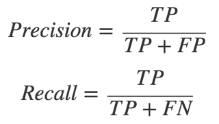
(where TP is the number of true positive results, FN is the number false negative, etc.)
The F-measure is the harmonic average between completeness and accuracy, and you can set the ratio with which these values are included in the result using the parameter ß:
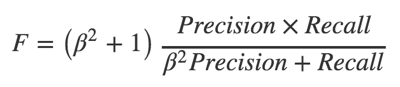
When ß> 1, the metric gets skewed towards completeness, with 0 <ß <1 - towards accuracy. We choose this parameter in accordance with the proportion of positive test sample examples for each subject at the current level, because the more vectors the classifier misses further, the more chances to make a mistake with the next one, and so on.
The next step is the calculation of the averaged F-measure for each independent branch of the tree, that is, for all the child nodes of the parent from the first level. Since for each node the F-measure was already calculated taking into account the composition of the training sample, it is sufficient to simply calculate the average F-measure of all the classifiers in the branch without additional weighting.
The single metric for the entire classifier is calculated as the weighted average of the branch metrics; weight is the proportion of positive branch examples in the sample. Here, a simple average is not enough; The number of nodes and search queries in different branches can vary greatly. We can boast a value of ~ 0.8 for the F-measure of the whole classifier, calculated in this way.
It is important to note that when testing a classifier, we remove the words of the corresponding search queries from the list of tokens in order to avoid feedback.
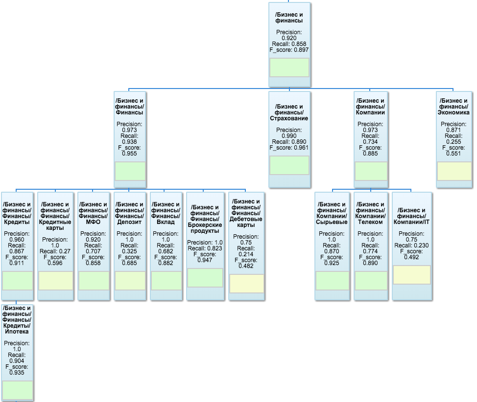
To visualize the test results, Google OrgChart is used - it first of all visually depicts the tree structure of the taxonomy, and also allows you to specify the values of metrics in each node and even hang the color indicators right inside the sheets. This is what one of the branches looks like:
The tester is implemented as a separate Flask application that loads pre-calculated metrics values from mongoDB on demand, completes what is missing due to possible changes in the classifier since the last calculation, and draws an orgchart. As a nice addition, a simple interface is available from there, allowing you to insert a list of URLs or plain text into the text field and look at the result of the classification.
Now, when there is a similar service, you need to actively use it. Every day, one million of the most visited sites of the last day are selected from our DMP and run through the classifier. These sites are marked with the id of the segments in which they fall, and users who have visited these pages in the last month fall into these segments. Now the classification of one page takes about 0.2 - 0.3 seconds (minus the latency of the hosting sites).
This approach allows you to automatically assign segments to thousands of URLs per day, whereas manually the analyst usually added no more than a hundred pages. Now the work of the analyst will be reduced only to the selection of suitable topics of search queries, DMP will do the rest for him and even will orient how well this has happened.
First of all, we were faced with the task of implementing a working classifier prototype, and at this stage we did not particularly bother with the choice of optimal parameters for estimators and other settings. However, we did not expect that such a rather simple mathematical model would show a quite decent quality of work. Of course, all the sounded algorithm constants can be flexibly adjusted, a separate article may be devoted to the selection of optimal settings. Now the plans include the following works:
We hope that the story was interesting. In the comments we will answer your questions and will be happy to discuss suggestions for improving our classifier.
42bcfae8-2ecc-438f-9e0b-841575de7479These numbers are keys in different tables, but the initial value is, first of all, the URL of the pages on which this cookie was downloaded, search queries, and sometimes some additional information that the provider gives - IP address, timestamp, customer information And so on. This data is rather heterogeneous, so the URL is the most valuable for segmentation. When creating a new segment, the analyst indicates a certain list of addresses, and if some cookie lights up on one of these pages, then it falls into the corresponding segment. It turns out that almost 90% of the working time of such analysts is spent on finding the right set of URLs - as a result of hard work with search engines, Yandex.Wordstat and other tools.
Having thus received more than a thousand segments, we realized that this process should be automated and simplified as much as possible, while being able to monitor the quality of the algorithms and provide analysts with a convenient interface for working with the new tool. Under the cut, I will tell you how we solve these problems.
So, as it was possible to understand from the introduction, in fact, it is not the users that need to be segmented, but the pages of Internet sites, - our analytic engine will automatically distribute users to the received segments.
It is worth saying a few words about how the segments are represented in our DMP. The main feature of a set of segments is that their structure is hierarchical, that is, is a tree. We do not impose any restrictions on the depth of the hierarchy, since each next level allows us to more accurately describe the portrait of the user's interests. Here are examples of several branches of the hierarchy:
')
If a user has visited a site that tells how to feed puppies or train a cat to the tray, it is likely that he is the owner of this animal, and it makes sense to show him the corresponding advertisements - about the veterinary clinic or a new line of feed. And if, before that, he chose premium brands in his online store, then he could have relatively high incomes, and he could advertise more expensive services - a feline psychologist or a canine barber.
In general, having some kind of manual taxonomy of the subject of Internet pages, it was necessary to create a service that, given an input URL, would output a list of topics suitable for it. We solve the problem of determining the subject of a web page as a multi-class classification according to the “one against all” scheme, that is, each classifier of its taxonomy has its own classifier. Classifiers are recursively bypassed, starting from the root of the topic tree and further down along those branches that are identified as suitable at each current level.
Device classifier
The frontend classifier is a Flask application, which holds an object in memory. In essence, it deals only with data preparation, deserialization of objects of trained classifiers of the class sklearn.ensemble.RandomForestClassifier stored in mongoDB, execution of their predict_proba () methods and processing of results in accordance with the existing taxonomy. Taxonomy with queries and test samples, by the way, is also stored in mongoDB.
The application waits for POST requests by the URI of the form:
- localhost / text /
- localhost / url /
- localhost / tokens /
classifier = RecursiveClassifier() app = Flask(__name__) @app.route("/text/", methods=['POST']) def get_text_topics(): data = json.loads(request.get_data().decode()) text = data['text'] return Response(json.dumps(classifier.get_text_topics(text), indent=4), mimetype='application/json') @app.route("/url/", methods=['POST']) def get_url_topics(): data = json.loads(request.get_data().decode()) url = data['url'] html = html_get(url) text = clean_html(html) return Response(json.dumps(classifier.get_text_topics(text,url), indent=4), mimetype='application/json') @app.route("/tokens/", methods=['POST']) def get_tokens_topics(): data = json.loads(request.get_data().decode()) return Response(json.dumps(classifier.get_tokens_topics(data), indent=4), mimetype='application/json') if __name__ == "__main__": app.run(host="0.0.0.0", port=config.server_port) Obtaining, for example, a certain URL, the application downloads its body, extracts the text directly from there, and initiates a recursive taxonomy traversal from the root to the children. Recursion occurs only for those nodes of the tree for which at the current step the probability of a page being owned by this node exceeds the threshold specified in the config.
Data preparation includes one-time tokenization of the text, calculation of the frequency characteristics of words and a feature conversion for each classifier in accordance with the weights for the tokens selected at the stage of the selection selection (more on this later). This uses the “ bag of words ” model, that is, the relative position of words in the text is ignored.
Training classifier
The learning process performs the backend. When changes are made to the taxonomy or to the list of requests for a node, the texts of new pages are downloaded and tokenized, then the learning algorithm is launched for all topics at the same level as the changed one. All the “brothers” of the classifier are retrained along with the changed, because the training sample for the whole level is the same - the texts of the sites from the TOP-50 Bing search results, found from all nodes of the brothers and all their children. For each topic, positive examples are sites that match their needs and the needs of their children, all other pages are negative examples. The result is stored in the pandas.DataFrame object.
The resulting sets of tokens with labels are then randomly distributed to the training sample (70%), the sample for the feature selection (15%) and the test sample (15%) - it is stored in mongoDB.
Feature selection
The selection of the most informative tokens is carried out in the learning process using the dg metric, and this is how it is implemented:
def dg(arr): avg = scipy.average(arr) summ = 0.0 for s in arr: summ += (s - avg) ** 2 summ /= len(arr) return math.sqrt(summ) / avg And this is how it is called for a set of tokens:
token_cnt = Counter() topic_cnt = Counter() topic_token_cnt = defaultdict(lambda: Counter()) for row in dataset.index: topic = dataset['topic'][row] topic_cnt[topic] += 1 for token in set(dataset['tokens'][row]): token_cnt[token] += 1 topic_token_cnt[topic][token] += 1 topics = list(topic_cnt.keys()) token_distr = {} for token in token_cnt: distr = [] for topic in topics: distr.append(topic_token_cnt[topic][token] / topic_cnt[topic]) token_distr[token] = distr token_dg = {} for token in token_distr: token_dg[token] = dg(token_distr[token]) * math.log(token_cnt[token]) Thus, the significance of words is assessed from the point of view of all texts of the training set. Since the frequency characteristics of the occurrence of words in the collection are used, it is interesting to look at the Zipf distribution . Here it is (green color shows linear interpolation of data):
Further, for vectorization of classified texts, including in the learning process, the weight obtained in this way is multiplied by the frequency of the word in this text, and 5 words are selected with the highest value of this value for each topic at a given taxonomy level. These vectors are further concatenated, resulting in a vector of length 5 * m, where m is the number of nodes in the level. Now the data is ready for classification.
Classifier quality assessment
We wanted to be able to get one number to evaluate the work of the entire classifier as a whole. It is clear that it is easy to calculate the accuracy, completeness and F-measure for each individual taxonomy node, but when more than one hundred classes come into it, there is little sense from this. Since the classifier is hierarchical, the quality of work of individual classifiers in the lower nodes depends on the quality of the previous ones - this is a key feature of our algorithm. Precision and Recall are calculated using the following formulas:
(where TP is the number of true positive results, FN is the number false negative, etc.)
The F-measure is the harmonic average between completeness and accuracy, and you can set the ratio with which these values are included in the result using the parameter ß:
When ß> 1, the metric gets skewed towards completeness, with 0 <ß <1 - towards accuracy. We choose this parameter in accordance with the proportion of positive test sample examples for each subject at the current level, because the more vectors the classifier misses further, the more chances to make a mistake with the next one, and so on.
The next step is the calculation of the averaged F-measure for each independent branch of the tree, that is, for all the child nodes of the parent from the first level. Since for each node the F-measure was already calculated taking into account the composition of the training sample, it is sufficient to simply calculate the average F-measure of all the classifiers in the branch without additional weighting.
The single metric for the entire classifier is calculated as the weighted average of the branch metrics; weight is the proportion of positive branch examples in the sample. Here, a simple average is not enough; The number of nodes and search queries in different branches can vary greatly. We can boast a value of ~ 0.8 for the F-measure of the whole classifier, calculated in this way.
It is important to note that when testing a classifier, we remove the words of the corresponding search queries from the list of tokens in order to avoid feedback.
To visualize the test results, Google OrgChart is used - it first of all visually depicts the tree structure of the taxonomy, and also allows you to specify the values of metrics in each node and even hang the color indicators right inside the sheets. This is what one of the branches looks like:
The tester is implemented as a separate Flask application that loads pre-calculated metrics values from mongoDB on demand, completes what is missing due to possible changes in the classifier since the last calculation, and draws an orgchart. As a nice addition, a simple interface is available from there, allowing you to insert a list of URLs or plain text into the text field and look at the result of the classification.
DMP Integration
Now, when there is a similar service, you need to actively use it. Every day, one million of the most visited sites of the last day are selected from our DMP and run through the classifier. These sites are marked with the id of the segments in which they fall, and users who have visited these pages in the last month fall into these segments. Now the classification of one page takes about 0.2 - 0.3 seconds (minus the latency of the hosting sites).
This approach allows you to automatically assign segments to thousands of URLs per day, whereas manually the analyst usually added no more than a hundred pages. Now the work of the analyst will be reduced only to the selection of suitable topics of search queries, DMP will do the rest for him and even will orient how well this has happened.
Future plans
First of all, we were faced with the task of implementing a working classifier prototype, and at this stage we did not particularly bother with the choice of optimal parameters for estimators and other settings. However, we did not expect that such a rather simple mathematical model would show a quite decent quality of work. Of course, all the sounded algorithm constants can be flexibly adjusted, a separate article may be devoted to the selection of optimal settings. Now the plans include the following works:
- We will transfer the classifier to the non-blocking Tornado server so that it can be accessed asynchronously;
- In addition to the dg metric, we consider various variations of tf-idf ;
- We will try to separately take into account the words that are contained in the title of the pages and meta tags;
- Twist the numerous estimator settings, try replacing random forest with SVM ensembles and increase the number of words selected for classification.
We hope that the story was interesting. In the comments we will answer your questions and will be happy to discuss suggestions for improving our classifier.
Source: https://habr.com/ru/post/261677/
All Articles