Analysis of the tone of statements on Twitter: implementation with an example of R
Social networks (Twitter, Facebook, LinkedIn) - perhaps the most popular free platform available to the general public for expressing thoughts on various occasions. Millions of tweets (posts) every day - there is a huge amount of information. In particular, Twitter is widely used by companies and ordinary people to describe the state of affairs, promote products or services. Twitter is also an excellent source of data for text mining: starting with the logic of behavior, events, the tone of statements and ending with the prediction of trends in the securities market. There is a huge array of information for intellectual and contextual analysis of texts.
In this article I will show how to conduct a simple analysis of the tonality of statements. We will upload twitter messages on a specific topic and compare them with a database of positive and negative words. The ratio of positive and negative words found is called the tonality ratio . We will also create functions for finding the most common words. These words can provide useful contextual information about public opinion and the tonality of statements. The data array for positive and negative words expressing opinions (tonal words) is taken from Hugh and Lew, KDD-2004 .
Implementing on R using
The first step is to register on the developer portal for Twitter and be authorized. You will need:
After receiving this data, log in to get access to the Twitter API:
')
The next step is to load an array of positive and negative tonal words (dictionary) into the working folder R. The words can be obtained from the variables,
Total 2006 positive and 4783 negative words. The section above also shows some examples of words from these dictionaries.
You can add new words to dictionaries or delete existing ones. Using the code below, we add the word
The next step is to set a search string for twitter messages and assign its value to a variable,
The code above uses the string "CyberSecurity" and 5,000 tweets. Twitter search code:
Tweets have many additional fields and system information. We use the
In this step, we will write a function that will execute a series of commands and clear the text: will remove punctuation, special characters, links, extra spaces, numbers. This function also causes uppercase and lowercase characters using
The clean () function clears tweets and breaks lines into word vectors.
In this step, we will use the
We got to the actual task of analyzing tweets. Compare the tweet texts with dictionaries and find matching words. In order to do this, we first define a function to count the positive and negative words that match the words from our database. Here is the
Now apply the function to the
The next step is to set a cycle for counting the total number of positive words in tweets.
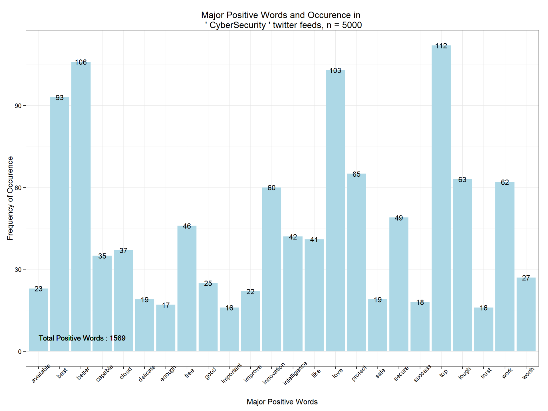
As seen above, there are 1569 positive words in tweets. Similarly, you can find the number of negative. The code below considers positive and negative entries.
This function is applied to the
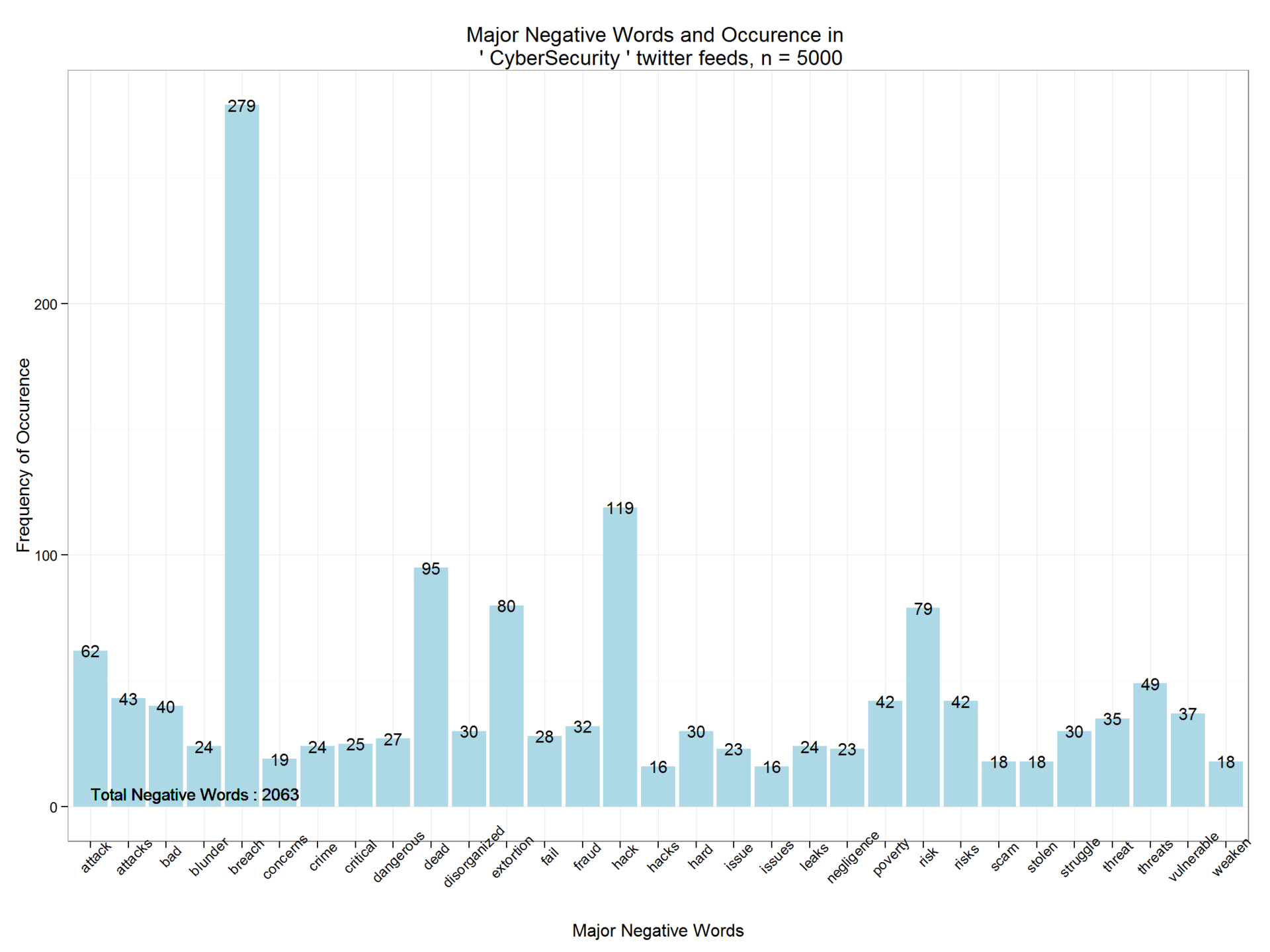
Similarly, a number of functions and cycles are created for counting negative tonal words. This information is recorded in another data frame,
In this section, we will create some graphs to show the distribution of frequently occurring negative and positive words. Use the
Using the
We will derive the main positive words and their frequency using the
Similarly, we derive negative words and their frequency. 5000 tweets containing the search string "CyberSecurity" contain 2,063 negative words.
Turn a
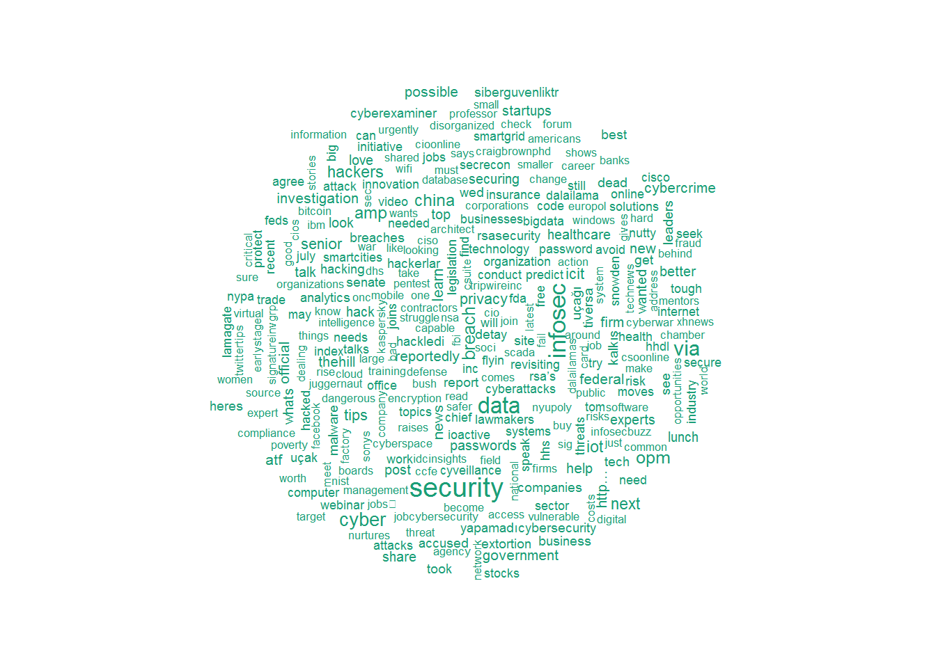
Now create a word cloud for tweets using the
In this final step, we turn the word block into a matrix of documents with the
Finally, we bring the matrix to the data frame, filter by the
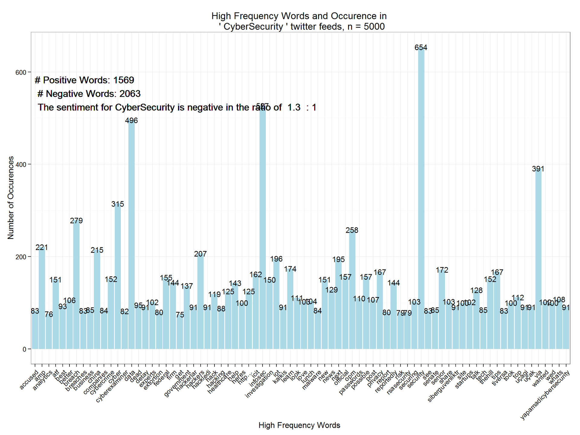
As you can see, the tonality of CyberSecurity is negative with a ratio of 1.3: 1. This analysis can be extended for several time intervals in order to highlight trends. You can also perform it iteratively, on similar topics, in order to compare and analyze the relative tonality rating.
In this article I will show how to conduct a simple analysis of the tonality of statements. We will upload twitter messages on a specific topic and compare them with a database of positive and negative words. The ratio of positive and negative words found is called the tonality ratio . We will also create functions for finding the most common words. These words can provide useful contextual information about public opinion and the tonality of statements. The data array for positive and negative words expressing opinions (tonal words) is taken from Hugh and Lew, KDD-2004 .
Implementing on R using
twitteR, dplyr, stringr, ggplot2, tm, SnowballC, qdap and wordcloud . Before use, you need to install and download these packages using the install.packages() and library() commands.Twitter API Download
The first step is to register on the developer portal for Twitter and be authorized. You will need:
api_key = " API" api_secret = " api_secret " access_token = " " access_token_secret = " " After receiving this data, log in to get access to the Twitter API:
setup_twitter_oauth(api_key,api_secret,access_token,access_token_secret) ')
Download dictionaries
The next step is to load an array of positive and negative tonal words (dictionary) into the working folder R. The words can be obtained from the variables,
positive and negative , as shown below. positive=scan('positive-words.txt',what='character',comment.char=';') negative=scan('negative-words.txt',what='character',comment.char=';') positive[20:30] ## [1] "accurately" "achievable" "achievement" "achievements" ## [5] "achievible" "acumen" "adaptable" "adaptive" ## [9] "adequate" "adjustable" "admirable" negative[500:510] ## [1] "byzantine" "cackle" "calamities" "calamitous" ## [5] "calamitously" "calamity" "callous" "calumniate" ## [9] "calumniation" "calumnies" "calumnious" Total 2006 positive and 4783 negative words. The section above also shows some examples of words from these dictionaries.
You can add new words to dictionaries or delete existing ones. Using the code below, we add the word
cloud to the positive dictionary and remove it from the negative dictionary. positive=c(positive,"cloud") negative=negative[negative!="cloud"] Search in twitter messages
The next step is to set a search string for twitter messages and assign its value to a variable,
findfd . The number of tweets to be used for analysis is assigned to another variable, number . The time for searching through messages and extracting information depends on this number. A slow internet connection or a complex search query can lead to delays. findfd= "CyberSecurity" number= 5000 The code above uses the string "CyberSecurity" and 5,000 tweets. Twitter search code:
tweet=searchTwitter(findfd,number) ## Time difference of 1.301408 mins Receiving text tweets
Tweets have many additional fields and system information. We use the
gettext() function to get the text fields and assign the resulting list to the variable tweetT . The feature applies to all 5,000 tweets. The code below also shows the result for the first five messages. tweetT=lapply(tweet,function(t)t$getText()) head(tweetT,5) ## [[1]] ## [1] "RT @PCIAA: \"You must have realtime technology\" how do you defend against #Cyberattacks? @FireEye #cybersecurity http://t.co/Eg5H9UmVlY" ## ## [[2]] ## [1] "@MPBorman: '#Cybersecurity on agenda for 80% corporate boards http://t.co/eLfxkgi2FT @CS… http://t.co/h9tjop0ete http://t.co/qiyfP94FlQ" ## ## [[3]] ## [1] "The FDA takes steps to strengthen cybersecurity of medical devices | @scoopit via @60601Testing http://t.co/9eC5LhGgBa" ## ## [[4]] ## [1] "Senior Solutions Architect, Cybersecurity, NYC-Long Island region, Virtual offic... http://t.co/68aOUMNgqy #job#cybersecurity" ## ## [[5]] ## [1] "RT @Cyveillance: http://t.co/Ym8WZXX55t #cybersecurity #infosec - The #DarkWeb As You Know It Is A Myth via @Wired http://t.co/R67Nh6Ck70" Text clearing function
In this step, we will write a function that will execute a series of commands and clear the text: will remove punctuation, special characters, links, extra spaces, numbers. This function also causes uppercase and lowercase characters using
tolower() . The tolower() function often fails if it encounters special characters and the code execution stops. To prevent this, we will write a function to intercept errors, tryTolower , and use it in the code of the text clearing function. tryTolower = function(x) { y = NA # tryCatch error try_error = tryCatch(tolower(x), error = function(e) e) # if not an error if (!inherits(try_error, "error")) y = tolower(x) return(y) } The clean () function clears tweets and breaks lines into word vectors.
clean=function(t){ t=gsub('[[:punct:]]','',t) t=gsub('[[:cntrl:]]','',t) t=gsub('\\d+','',t) t=gsub('[[:digit:]]','',t) t=gsub('@\\w+','',t) t=gsub('http\\w+','',t) t=gsub("^\\s+|\\s+$", "", t) t=sapply(t,function(x) tryTolower(x)) t=str_split(t," ") t=unlist(t) return(t) } Clearing and splitting tweets into words
In this step, we will use the
clean() function to clear 5000 tweets. The result will be stored in the tweetclean list tweetclean . The following code also shows the first five tweets cleared and broken into words using this function. tweetclean=lapply(tweetT,function(x) clean(x)) head(tweetclean,5) ## [[1]] ## [1] "rt" "pciaa" "you" "must" ## [5] "have" "realtime" "technology" "how" ## [9] "do" "you" "defend" "against" ## [13] "cyberattacks" "fireeye" "cybersecurity" ## ## [[2]] ## [1] "mpborman" "cybersecurity" "on" "agenda" ## [5] "for" "" "corporate" "boards" ## [9] " " "cs" ## ## [[3]] ## [1] "the" "fda" "takes" "steps" ## [5] "to" "strengthen" "cybersecurity" "of" ## [9] "medical" "devices" "" "scoopit" ## [13] "via" "testing" ## ## [[4]] ## [1] "senior" "solutions" "architect" ## [4] "cybersecurity" "nyclong" "island" ## [7] "region" "virtual" "offic" ## [10] "" "jobcybersecurity" ## ## [[5]] ## [1] "rt" "cyveillance" "" "cybersecurity" ## [5] "infosec" "" "the" "darkweb" ## [9] "as" "you" "know" "it" ## [13] "is" "a" "myth" "via" ## [17] "wired" Tweet analysis
We got to the actual task of analyzing tweets. Compare the tweet texts with dictionaries and find matching words. In order to do this, we first define a function to count the positive and negative words that match the words from our database. Here is the
returnpscore function returnpscore for counting positive matches. returnpscore=function(tweet) { pos.match=match(tweet,positive) pos.match=!is.na(pos.match) pos.score=sum(pos.match) return(pos.score) } Now apply the function to the
tweetclean list. positive.score=lapply(tweetclean,function(x) returnpscore(x)) The next step is to set a cycle for counting the total number of positive words in tweets.
pcount=0 for (i in 1:length(positive.score)) { pcount=pcount+positive.score[[i]] } pcount ## [1] 1569 As seen above, there are 1569 positive words in tweets. Similarly, you can find the number of negative. The code below considers positive and negative entries.
poswords=function(tweets){ pmatch=match(t,positive) posw=positive[pmatch] posw=posw[!is.na(posw)] return(posw) } This function is applied to the
tweetclean list, and in the loop, words are added to the data frame, pdatamart . The code below shows the first 10 occurrences of positive words. words=NULL pdatamart=data.frame(words) for (t in tweetclean) { pdatamart=c(poswords(t),pdatamart) } head(pdatamart,10) ## [[1]] ## [1] "best" ## ## [[2]] ## [1] "safe" ## ## [[3]] ## [1] "capable" ## ## [[4]] ## [1] "tough" ## ## [[5]] ## [1] "fortune" ## ## [[6]] ## [1] "excited" ## ## [[7]] ## [1] "kudos" ## ## [[8]] ## [1] "appropriate" ## ## [[9]] ## [1] "humour" ## ## [[10]] ## [1] "worth" Similarly, a number of functions and cycles are created for counting negative tonal words. This information is recorded in another data frame,
ndatamart . Here is a list of the first ten negative words in tweets. head(ndatamart,10) ## [[1]] ## [1] "attacks" ## ## [[2]] ## [1] "breach" ## ## [[3]] ## [1] "issues" ## ## [[4]] ## [1] "attacks" ## ## [[5]] ## [1] "poverty" ## ## [[6]] ## [1] "attacks" ## ## [[7]] ## [1] "dead" ## ## [[8]] ## [1] "dead" ## ## [[9]] ## [1] "dead" ## ## [[10]] ## [1] "dead" Graphs of frequently occurring negative and positive words
In this section, we will create some graphs to show the distribution of frequently occurring negative and positive words. Use the
unlist() function to turn lists into vectors. The vector variables pwords and nwords are nwords to data frame objects. dpwords=data.frame(table(pwords)) dnwords=data.frame(table(nwords)) Using the
dplyr package, you need to bring words to character type variables and then filter out positive and negative for frequency ( frequency > 15 ). dpwords=dpwords%>% mutate(pwords=as.character(pwords))%>% filter(Freq>15) We will derive the main positive words and their frequency using the
ggplot2 package. As you can see, positive words are only 1569. The distribution function shows the degree of positive tonality. ggplot(dpwords,aes(pwords,Freq))+geom_bar(stat="identity",fill="lightblue")+theme_bw()+ geom_text(aes(pwords,Freq,label=Freq),size=4)+ labs(x="Major Positive Words", y="Frequency of Occurence",title=paste("Major Positive Words and Occurence in \n '",findfd,"' twitter feeds, n =",number))+ geom_text(aes(1,5,label=paste("Total Positive Words :",pcount)),size=4,hjust=0)+theme(axis.text.x=element_text(angle=45)) Similarly, we derive negative words and their frequency. 5000 tweets containing the search string "CyberSecurity" contain 2,063 negative words.
Delete common words and create a word cloud
Turn a
tweetclean into a word block using the VectorSource function. Block representation will remove redundant common words with the text mining package tm . Removing common words, so-called stop words, will help us focus on the important and highlight the context. The code below displays several examples of stop words: tweetscorpus=Corpus(VectorSource(tweetclean)) tweetscorpus=tm_map(tweetscorpus,removeWords,stopwords("english")) stopwords("english")[30:50] ## [1] "what" "which" "who" "whom" "this" "that" "these" ## [8] "those" "am" "is" "are" "was" "were" "be" ## [15] "been" "being" "have" "has" "had" "having" "do" Now create a word cloud for tweets using the
wordcloud package. Please note we limit the maximum amount to 300. wordcloud(tweetscorpus,scale=c(5,0.5),random.order = TRUE,rot.per = 0.20,use.r.layout = FALSE,colors = brewer.pal(6,"Dark2"),max.words = 300) Analyzing and plotting common words
In this final step, we turn the word block into a matrix of documents with the
DocumentTermMatrix function. The matrix of documents can be analyzed for frequently encountered atypical words. Then we remove rare words from the block (with a too low frequency of occurrence). The code below displays the most common ones (with a frequency of 50 or higher). dtm=DocumentTermMatrix(tweetscorpus) # #removing sparse terms dtms=removeSparseTerms(dtm,.99) freq=sort(colSums(as.matrix(dtm)),decreasing=TRUE) #get some more frequent terms findFreqTerms(dtm,lowfreq=100) ## [1] "amp" "atf" "better" "breach" ## [5] "china" "cyber" "cybercrime" "cybersecurity" ## [9] "data" "experts" "federal" "firm" ## [13] "government" "hackers" "hack" "healthcare" ## [17] "help" "heres" "http…" "icit" ## [21] "infosec" "investigation" "iot" "learn" ## [25] "look" "love" "lunch" "new" ## [29] "news" "next" "official" "opm" ## [33] "passwords" "possible" "post" "privacy" ## [37] "reportedly" "securing" "security" "senior" ## [41] "share" "site" "startups" "talk" ## [45] "thehill" "tips" "took" "top" ## [49] "via" "wanted" "wed" "whats" Finally, we bring the matrix to the data frame, filter by the
Minimum frequency > 75 and plot the graph using ggplot2 : wf=data.frame(word=names(freq),freq=freq) wfh=wf%>% filter(freq>=75,!word==tolower(findfd)) ggplot(wfh,aes(word,freq))+geom_bar(stat="identity",fill='lightblue')+theme_bw()+ theme(axis.text.x=element_text(angle=45,hjust=1))+ geom_text(aes(word,freq,label=freq),size=4)+labs(x="High Frequency Words ",y="Number of Occurences", title=paste("High Frequency Words and Occurence in \n '",findfd,"' twitter feeds, n =",number))+ geom_text(aes(1,max(freq)-100,label=paste("# Positive Words:",pcount,"\n","# Negative Words:",ncount,"\n",result(ncount,pcount))),size=5, hjust=0) findings
As you can see, the tonality of CyberSecurity is negative with a ratio of 1.3: 1. This analysis can be extended for several time intervals in order to highlight trends. You can also perform it iteratively, on similar topics, in order to compare and analyze the relative tonality rating.
Source: https://habr.com/ru/post/261589/
All Articles