Automatic reorganization of arrays in the memory of the graphics accelerator

What are we talking about

In this post I would like to describe a part of the runtime system (RTS - RunTime System hereinafter) of the DVMH compiler. The considered part, as can be seen from the title, relates to the processing of user arrays on the GPU, namely, their automatic transformation or reorganization in the memory of the accelerator. These transformations are done for efficient access to the GPU memory in computational cycles. What is DVMH, how to adjust to the calculations and why it is done automatically - described below.

What is DVMH

Since this post is devoted to the review of algorithms for the transformation of arrays, I will describe only briefly what DVMH is, as it will be needed to describe the principles of operation. We need to start with a DVM (Distribute Virtual Memory) system - with a system that is designed to develop programs for clusters containing accelerators in nodes (GPU Nvidia and Intel Xeon Phi) and multi-core processors. With this system, you can easily parallelize large sequential programs that work primarily with structural grids or structural data types, and also easily display a program on a cluster, in the nodes of which there can be devices of different architectures. DVM-system includes:

Compilers from C programming languages (and in the future C ++, with some limitations, of course) and Fortran C-DVMH and Fortran-DVMH. We will call generically DVMH languages and compilers. DVMH is an extension of the considered programming languages by pragmas or special comments that are not visible to standard compilers (by analogy, for example, with OpenMP, OpenACC). Thus, it is enough for a programmer to place a small number of directives indicating how the data is distributed and how calculations are displayed on the distributed data in the computational cycles. After that, the user receives both a sequential program and a parallel program. The resulting program can be run on a cluster on a different number of nodes, on one or several GPUs within one node, and also, for example, use multi-core processors, graphics accelerators and Intel Xeon Phi accelerators at once (if all this is present on the server in question). More details can be found here;
Lib-DVMH support library or RTSH run-time system (H means heterogeneous, this letter in the name of many components appeared after the system was expanded to support GPU and Xeon Phi). With the help of this system, the entire user program setup is performed while the program is running;
Debugging tools and debugging tools for the effectiveness of DVMH programs (currently only for Fortran-DVMH programs).

The main goal of creating such a system is to simplify the user’s life by paralleling existing programs and simplify the writing of new parallel programs. DVMH compilers translate the resulting program with DVMH directives into a program using MPI, OpenMP and CUDA and RTSH calls. Thus, a user program can be easily parallelized with the help of calculation distribution directives (almost similar to OpenMP or OpenACC) and data distribution directives. Moreover, this program continues to be consistent, which is important for its further development and support. It is still easier to write a “good” sequential program and place directives in the DVMH compiler in such a program, than doing manual parallelization.

Concurrency levels

After a brief introduction and introduction to the course of the matter, let us consider how the source program (namely, computational cycles) is mapped to different levels of parallelism inside the RTSH. Currently, in order to achieve a large computing power, a large number of threads are used within a single device, instead of increasing the frequency of operation of each of the threads. This in turn leads to the need to study not only the standard (MPI of course) interaction of processes between nodes, but also the emergence of heterogeneous architectures, and with them various parallel languages, both high-level and low-level. And all this makes life difficult for the end user. And in order to achieve high application performance, it is necessary to use all the capabilities of a specific computing cluster.
')
At the moment, you can imagine two levels of parallelism - between nodes and within a node. Inside the node can be used one or more GPU, as well as multi-core processors. Intel Xeon Phi in this scheme is considered as a separate node containing a multi-core processor. Below is a generalized diagram of a computing cluster on which DVMH programs can be mapped:

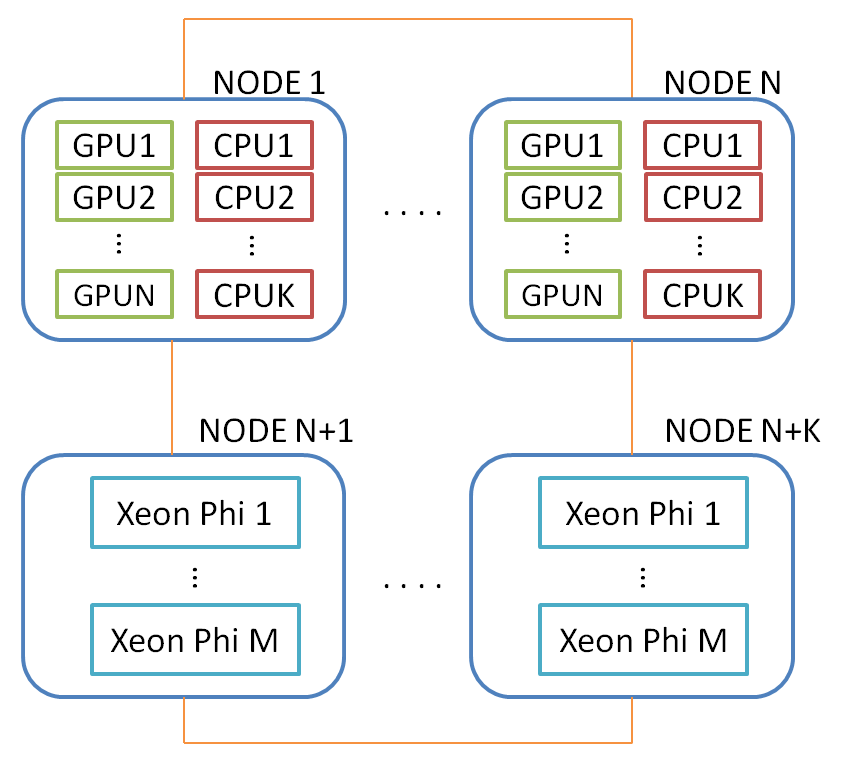
Naturally, the question arises of balancing the loading of devices (the mechanism of which is in DVMH), but this is already beyond the scope of this post. All further considerations will affect a single GPU within a single node. The following transformations are performed on all GPUs on which the DVMH program runs, independently.

What is data reorganization necessary for?

Finally, after a protracted entry, we come to the question of the reorganization itself. What is all this for? But for what. Consider some kind of computational cycle:

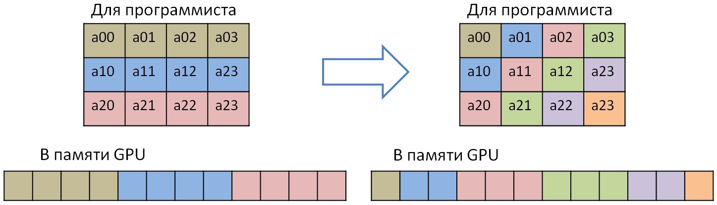
double ARRAY[Z][Y][X][5]; for(int I = 1; i < Z; ++I) for(int J = 1; J < Y; ++J) for(int K = 1; K < X; ++K) ARRAY[K][J][I][4] = Func(ARRAY[K][J][I][2], ARRAY[K][J][I][5]);

We have a four-dimensional array, where the first (fastest) measurement, for example, contains 5 physical quantities, and the rest are coordinates in the space of the computational domain. In the program, the array was declared so that the first (close-in-memory) dimension consists of these 5 elements so that the processor cache works well in computational cycles. In this example, you need access to 2, 4 and 5 fast measurement elements at each iteration of three cycles. It is also worth noting that there is no cycle for this measurement. And by virtue of, for example, the different nature of these quantities, the calculations for each of the 5 elements will also differ.

Thus, it is possible to execute parallel cycles for I, J, K. For this example, each element of the ARRAY array will be somehow mapped onto a parallel loop, for example, like this:

 #pragma dvm array distribute[block][block][block][*] double ARRAY[Z][Y][X][5]; #pragma dvm parallel([I][J][K] on ARRAY[I][J][K][*]) for(int I = 1; i < Z; ++I) for(int J = 1; J < Y; ++J) for(int K = 1; K < X; ++K) ARRAY[K][J][I][4] = Func(ARRAY[K][J][I][2], ARRAY[K][J][I][5]);

That is, a data distribution appears, in relation to which the calculations are distributed. The above DVMH directives suggest that the array should be distributed in three dimensions in equal blocks, and the fourth (fastest) should be propagated. This record allows you to display an array on the processor grid specified when the DVMH program was started. The following directive says that it is necessary to perform a round (I, J, K) in accordance with the rule of distribution of the array ARRAY. Thus, the PARALLEL directive sets the display of the loop turns on the array elements. At run time, the RTSH knows how the arrays are located and how to organize the calculations.

This cycle, namely the entire space of the turns, can be displayed both on the OpenMP thread and on the CUDA thread, because all three cycles have no dependencies. We are interested in mapping on CUDA architecture. Everyone knows that the CUDA block contains three dimensions - x, y, z. The very first is the fastest. Fast measurement is displayed on the warp'y CUDA-block. Why should all this be mentioned? Because the global GPU memory (GDDR5) is a bottleneck in any computing. And the memory is arranged in such a way that the fastest access is carried out by one warp only if all the loaded elements lie in a row. For the above cycle, there are 6 options for mapping the space of turns (I, J, K) to the CUDA block (x, y, z), but none of them allows you to effectively access the ARRAY array.

What does it come from? If you look at the description of the array, you can see that the first dimension contains 5 elements and there is no cycle for it. Thus, the elements of the second fast measurement lie at a distance of 40 bytes (5 elements of the double type), which leads to an increase in the number of transactions to the GPU memory (instead of 1 transaction, one warp can do up to 32 transactions). All this leads to an overload of the memory bus and a decrease in performance.

To solve the problem, in this case, it is enough to swap the first and second measurements, that is, to transpose the two-dimensional matrix of X * 5 Y * Z times or perform Y * Z independent transpositions. But what does swapping array measurements mean? The following problems may occur:

It is necessary to add additional cycles to the code that perform this conversion;
If you rearrange the measurements in the program code, you will have to correct the entire program, since the calculations in all cycles will become incorrect if you rearrange the measurements of the array at one point of the program. And if the program is large, then you can make a lot of mistakes;
It is not clear what effect of the permutation will be obtained and how the permutation will affect another cycle. It is quite possible that you need a new permutation or the return of the array to its initial state
Create two versions of the program, since this cycle will cease to run efficiently on the CPU.

Implement various permutations in the RTSH

To solve the problems described in RTSH, an automatic array transformation mechanism was invented, which allows the user’s DVMH program to be significantly accelerated (several times) in case of unsuccessful access to the GPU memory (compared to its execution without using this feature). Before considering the types of transformation and their implementation on CUDA, I will list some of the undeniable advantages of our approach:

The user has one DVMH program, he focuses on writing an algorithm;
This mode can be enabled during compilation of a DVMH program by specifying just one DVMH option to the -autoTfm compiler. Thus, the user can try both modes without any changes to the program and evaluate the acceleration;
This transformation is performed in the "on demand" mode. This means that in the case of a change in the order of measurements of the array before the computational cycle, the inverse permutation will not be performed after the calculations, since it is quite possible that this arrangement of the array will be beneficial for the next cycle;
Significant acceleration of the program (up to 6 times) compared with the same program, performed without the use of this option.

1. Swap the array measurements that are physically adjacent.

The example described above fits this type of conversion. In this case, it is necessary to transpose the two-dimensional plane, which can be located on any adjacent two dimensions of the array. If it is necessary to transpose the first two dimensions, then a well-described matrix transposition algorithm using shared memory is suitable:

 __shared__ T temp[BLOCK_DIM][BLOCK_DIM + 1]; CudaSizeType x1Index = (blockIdx.x + pX) * blockDim.x + threadIdx.x; CudaSizeType y1Index = (blockIdx.y + pY) * blockDim.y + threadIdx.y; CudaSizeType x2Index = (blockIdx.y + pY) * blockDim.y + threadIdx.x; CudaSizeType y2Index = (blockIdx.x + pX) * blockDim.x + threadIdx.y; CudaSizeType zIndex = blockIdx.z + pZ; CudaSizeType zAdd = zIndex * dimX * dimY; CudaSizeType idx1 = x1Index + y1Index * dimX + zAdd; CudaSizeType idx2 = x2Index + y2Index * dimY + zAdd; if ((x1Index < dimX) && (y1Index < dimY)) { temp[threadIdx.y][threadIdx.x] = inputMatrix[idx1]; } __syncthreads(); if ((x2Index < dimY) && (y2Index < dimX)) { outputMatrix[idx2] = temp[threadIdx.x][threadIdx.y]; }

In the case of a square matrix, you can perform the transposition of the so-called "in place", for which you do not need to allocate additional memory on the GPU.

2. Swap the array measurements that are not physically adjacent.

This type includes permutations of any two dimensions of the array. It is necessary to distinguish two types of such permutations: the first is to change any measurement with the first and change any measurements between them, and neither is the first (fastest) one. This separation should be clear, since the elements of the fastest measurement lie in a row and access to them should also be possible in a row. To do this, you can use shared memory:

 __shared__ T temp[BLOCK_DIM][BLOCK_DIM + 1]; CudaSizeType x1Index = (blockIdx.x + pX) * blockDim.x + threadIdx.x; CudaSizeType y1Index = (blockIdx.y + pY) * blockDim.y + threadIdx.y; CudaSizeType x2Index = (blockIdx.y + pY) * blockDim.y + threadIdx.x; CudaSizeType y2Index = (blockIdx.x + pX) * blockDim.x + threadIdx.y; CudaSizeType zIndex = blockIdx.z + pZ; CudaSizeType zAdd = zIndex * dimX * dimB * dimY; CudaSizeType idx1 = x1Index + y1Index * dimX * dimB + zAdd; CudaSizeType idx2 = x2Index + y2Index * dimY * dimB + zAdd; for (CudaSizeType k = 0; k < dimB; k++) { if (k > 0) __syncthreads(); if ((x1Index < dimX) && (y1Index < dimY)) { temp[threadIdx.y][threadIdx.x] = inputMatrix[idx1 + k * dimX]; } __syncthreads(); if ((x2Index < dimY) && (y2Index < dimX)) { outputMatrix[idx2 + k * dimY] = temp[threadIdx.x][threadIdx.y]; } }

If you need to perform a permutation of any other measurements among themselves, then the shared memory is not needed, since access to the fast measurement of the array will be performed “correctly” (the neighboring threads will work with the neighboring cells in the GPU memory).

3. Perform diagonalization of the array.

This type of permutation is non-standard and is necessary for parallel execution of loops with regular data dependency. This permutation provides “correct” access when processing a loop in which there are dependencies. Consider an example of such a cycle:

 #pragma dvm parallel([ii][j][i] on A[i][j][ii]) across(A[1:1][1:1][1:1]) for (ii = 1; ii < K - 1; ii++) for (j = 1; j < M - 1; j++) for (i = 1; i < N - 1; i++) A[i][j][ii] = A[i + 1][j][ii] + A[i][j + 1][ii] + A[i][j][ii + 1] + A[i - 1][j][ii] + A[i][j - 1][ii] + A[i][j][ii - 1];

In this case, there is a dependency on all three dimensions of the cycle or three dimensions of array A. To tell the DVMH compiler that there is a regular dependency in this cycle (dependent elements can be expressed by the formula a * x + b, where a and b are constants), there is an ACROSS specification. In this cycle there are direct and inverse dependencies. The space of turns of this cycle form a parallelepiped (and in the particular case - a three-dimensional cube). The planes of this parallelepiped, rotated at 45 degrees relative to each face, can be carried out in parallel, while the planes themselves can be performed sequentially. Because of this, access to the diagonal elements of the first two fastest measurements of the array A appears. And in order to increase the performance of the GPU, it is necessary to perform a diagonal transformation of the array. In the simple case, the transformation of one plane looks like this:

You can perform this transformation as fast as matrix transposition. To do this, you must use shared memory. Only unlike matrix transposition, the processed block will not be square, but in the form of a parallelogram, so that when reading and writing efficiently use the memory bandwidth of the GPU (only the first band is shown for diagonalization, since all the others are broken down in a similar way):

The following diagonalization types have been implemented (Rx and Ry are the sizes of the diagonalizable rectangle):

Parallel to the secondary diagonal and Rx == Ry;
Parallel to the secondary diagonal and Rx <Ry;
Parallel to the secondary diagonal and Rx> Ry;
Parallel to the main diagonal and Rx == Ry;
Parallel to the main diagonal and Rx <Ry;
Parallel to the main diagonal and Rx> Ry.

The common core for diagonalization is as follows:

 __shared__ T data[BLOCK_DIM][BLOCK_DIM + 1]; __shared__ IndexType sharedIdx[BLOCK_DIM][BLOCK_DIM + 1]; __shared__ bool conditions[BLOCK_DIM][BLOCK_DIM + 1]; bool condition; IndexType shift; int revX, revY; if (slash == 0) { shift = -threadIdx.y; revX = BLOCK_DIM - 1 - threadIdx.x; revY = BLOCK_DIM - 1 - threadIdx.y; } else { shift = threadIdx.y - BLOCK_DIM; revX = threadIdx.x; revY = threadIdx.y; } IndexType x = (IndexType)blockIdx.x * blockDim.x + threadIdx.x + shift; IndexType y = (IndexType)blockIdx.y * blockDim.y + threadIdx.y; IndexType z = (IndexType)blockIdx.z * blockDim.z + threadIdx.z; dvmh_convert_XY<IndexType, slash, cmp_X_Y>(x, y, Rx, Ry, sharedIdx[threadIdx.y][threadIdx.x]); condition = (0 <= x && 0 <= y && x < Rx && y < Ry); conditions[threadIdx.y][threadIdx.x] = condition; if (back == 1) __syncthreads(); #pragma unroll for (int zz = z; zz < z + manyZ; ++zz) { IndexType normIdx = x + Rx * (y + Ry * zz); if (back == 0) { if (condition && zz < Rz) data[threadIdx.y][threadIdx.x] = src[normIdx]; __syncthreads(); if (conditions[revX][revY] && zz < Rz) dst[sharedIdx[revX][revY] + zz * Rx * Ry] = data[revX][revY]; } else { if (conditions[revX][revY] && zz < Rz) data[revX][revY] = src[sharedIdx[revX][revY] + zz * Rx * Ry]; __syncthreads(); if (condition && zz < Rz) dst[normIdx] = data[threadIdx.y][threadIdx.x]; } }

In this case, it is necessary to transfer the condition value and the calculated coordinate in the diagonal representation with the help of dvmh_convert_XY to other threads, because unlike transposition, it is not possible here to unambiguously calculate both coordinates (where to read and where to write).

Total. What permutations are implemented:

Rearrange two adjacent array dimensions;
Rearrange two non-adjacent array dimensions;
Digalization of two adjacent fastest array measurements;
[Planned] Digonization of any two fastest array measurements (diagonalizable measurement becomes the fastest);
Copying the clipping from the diagonalized array (for example, to update the “shadow” edges in the case of an account on several GPUs);

Performance evaluation

To demonstrate the effectiveness of the approach, I will cite some graphs showing the performance of the permutations themselves and give the results of two programs - LU decomposition for the gas hydrodynamics problem and a synthetic test that implements the method of sequential upper relaxation for solving the 3-dimensional Dirichlet problem. All tests were run on GPU GTX Titan and Nvidia CUDA ToolKit 7.0 and Intel Xeon E5 1660 v2 processor with Intel compiler version 15.

We will compare all the implemented transformations with the usual copy core, since the reorganization of arrays is a copying of one memory section to another according to a certain rule. The copy kernel looks like this:

 __global__ void copyGPU(const double *src, double *dist, unsigned elems) { unsigned idx = blockIdx.x * blockDim.x + threadIdx.x; if(idx < elems) dist[idx] = src[idx]; }

I will give the conversion speed only for algorithms that use shared memory, as in this case there is an additional overhead of synchronization inside the CUDA block, as well as access to shared memory (L1 cache), because of which the performance of such copying will be lower than with any other permutations. We take the copyGPU copying speed as 100%, since in this case the overhead is minimal and this core allows getting almost peak memory bandwidth of the GPU.

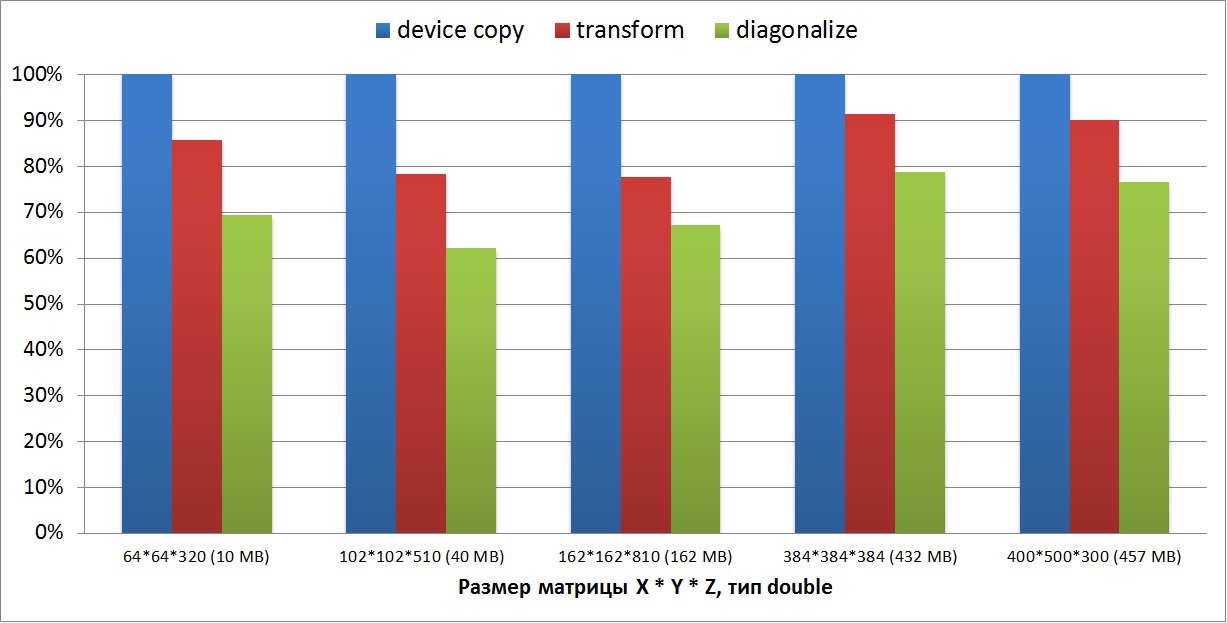
The first graph shows how much slower the transformation (transposition) and the diagonalization of the two-dimensional matrix were performed. The size of the matrix varies from a few megabytes to one gigabyte. From the graph it can be seen that on two-dimensional matrices the performance drop is 20-25% relative to the copyGPU core. You can also see that the diagonalization is performed by 5% longer, since the diagonalization algorithm is somewhat more complicated than matrix transposition:

The second graph shows how much slower the transformation (transposition) and the diagonalization of the three-dimensional matrix were performed. The dimensions of the matrices were taken in two types: four-dimensional N * N * N * 5 and arbitrary X * Y * Z. Matrix sizes range from 10 megabytes to 500 megabytes. On small matrices, the conversion speed drops by 40%, while on large matrices, the transformation speed reaches 90%, and the diagonalization speed, 80% of the copy speed:

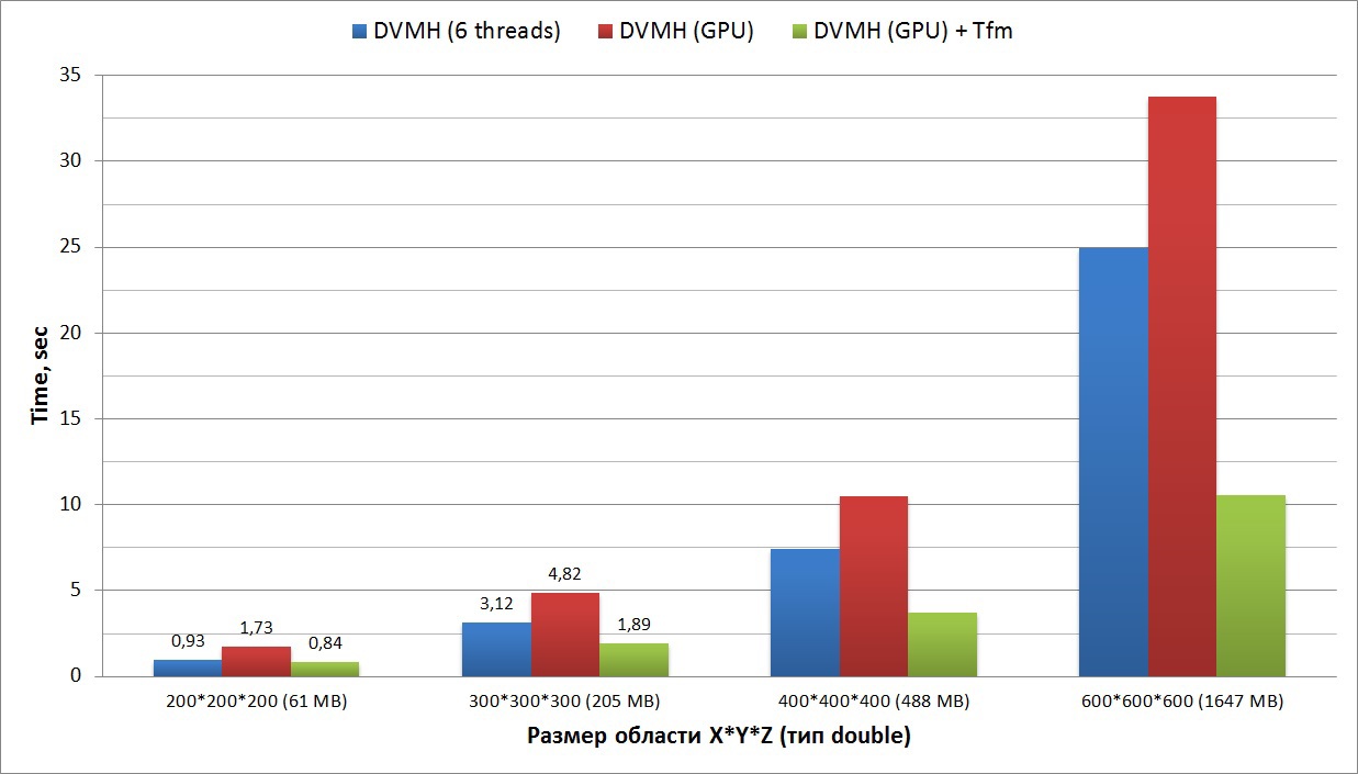
The third graph shows the execution time of a synthetic test that implements the symmetrical upper relaxation method. The computational cycle of this method contains dependencies in all three dimensions (this cycle is described in C language above). The graph shows the execution times of the same DVMH program (written in Fortran, the source code is attached at the end of the article), using 6 threads of Xeon E5 and on the GPU using diagonalization and without. In this case, the diagonalization must be done only once before the iterative calculations.

The fourth graph shows the acceleration of an application that solves a synthetic system of nonlinear partial differential equations (3-D Navier-Stokes equations for compressible fluid or gas) using the symmetric sequential upper relaxation method (SSOR algorithm, LU problem). This test is part of the standard NASA test suite (latest available version 3.3.1). In this set, the source codes of all tests of successive versions are available, as well as MPI and OpenMP.

The graph shows the acceleration of the program with respect to the serial version, performed on one Xeon E5 core, performed on 6 threads of Xeon E5, and on the GPU in two modes. In this program, it is necessary to do diagonalization only for two cycles, and then return the array to its original state, that is, at each iteration for “bad” cycles, all the required arrays are diagonalized, and after execution it occurs from the diagonalization. It is also worth noting that in this program about 2500 thousand lines of Fortran 90 style (without hyphenation, the code at the end of the article is attached). 125 DVMH-directives are added to it, which allow you to execute this program both on a cluster, on a single node on different devices, and in sequential mode.

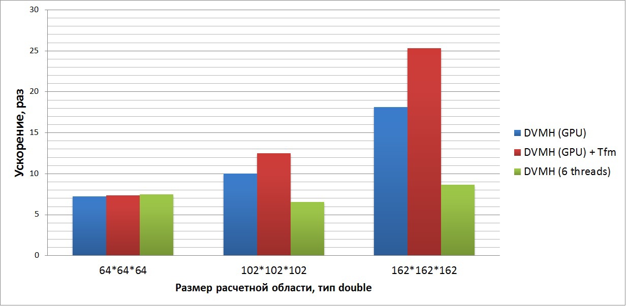
This program is well optimized at the level of sequential code (this is evident from the 8-fold acceleration on 6 Xeon E5 cores), which is well reflected not only on the GPU architecture, but also on multi-core processors. The DVMH compiler allows using the -Minfo option to see the number of registers required by the CUDA cores corresponding to each displayed cycle (this information is taken from the Nvidia compiler). In this case, you need about 160 registers per thread (out of 255 available) for each of the three main computational cycles, and the number of operations to access global memory is approximately 10: 1. Thus, the acceleration from the use of reorganization is not so great, but it is still there and on a large task it is 1.5 times as compared with the same program executed without this option. Also, this test is performed 3 times faster on the GPU than on the 6 CPU cores.

Conclusion

In this post, an approach was considered to automatically reorganize data on the GPU in the support system for DVMH programs. In this case, we are talking about the full automation of this process. RTSH has all the information during program execution that is necessary to determine the type of reorganization. This approach allows you to get a good acceleration on those programs where you can not write a "good" sequential program, while displaying the cycles of which access to the global memory of the GPU was carried out in the best way. When performing transformations, up to 90% of the performance of global GPU memory (which is approximately 240 GB / s for GTX Titan) is achieved relative to the fastest memory copy core inside the device.