Content

1. What is a tensor and what is it for?
2. Vector and tensor operations. Ranks of tensors
3. Curved coordinates
4. Dynamics of a point in the tensor representation
5. Actions on tensors and some other theoretical questions
6. Kinematics of free solid. Nature of angular velocity
7. The final turn of a solid. Rotation tensor properties and method for calculating it
8. On convolutions of the Levi-Civita tensor
9. Conclusion of the angular velocity tensor through the parameters of the final rotation. Apply head and maxima
10. Get the angular velocity vector. We work on the shortcomings
11. Acceleration of the point of the body with free movement. Solid Corner Acceleration
12. Rodrig – Hamilton parameters in solid kinematics
13. SKA Maxima in problems of transformation of tensor expressions. Angular velocity and acceleration in the parameters of Rodrig-Hamilton
14. Non-standard introduction to solid body dynamics
15. Non-free rigid motion
16. Properties of the inertia tensor of a solid
17. Sketch of nut Janibekov
18. Mathematical modeling of the Janibekov effect

Introduction

It was a long time ago when I was in the tenth grade. Among the rather scientifically scientifically scientifically-owned fund of the district library I came across a book - V. Ugarov, “The Special Theory of Relativity.” This topic interested me at that time, but the information from school textbooks and reference books was not enough.
')
However, I could not read this book, for the reason that most of the equations were represented there in the form of tensor relations. Later, at the university, the training program in my specialty did not provide for the study of tensor calculus, although the incomprehensible term “tensor” appeared quite often in some special courses. For example, it was terribly incomprehensible why a matrix containing moments of inertia of a solid body is proudly referred to as the inertia tensor.

Immersion in the special literature did not bring enlightenment. Techie hard enough to digest a strict abstract language of pure mathematics. However, from time to time I returned to this issue, and now, after almost sixteen years, there was enlightenment, which will be discussed under the cut. Perhaps my reasoning will seem primitive and simplistic, but the understanding of any complex thing is taken from the process of operating with simple concepts, so let's begin.

1. A vector on a plane. Contravariant, covariant coordinates and the relationship between them

Consider the vector, and without loss of generality of our reasoning, consider the vector defined on the plane. As it is known from the course of school geometry, any vector can be defined on the plane using two non-collinear vectors.



Here - decomposition coefficients, (the superscript should be understood to mean the number of the component, and not the return to the power), called the countervariant coordinates of the vector . Geometrically, this can be represented as shown in the figure below. Vectors called the base angle between them, provided , may be arbitrary, arbitrary as well non-zero length of the basis vectors. The specified basis specifies an oblique coordinate system on the plane, with the axes .



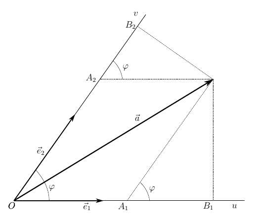
Based on the drawing lengths of segments and are equal



However, this is not the only way to define a vector. in this coordinate system. It can also be specified by orthogonal projections on the axes. . It is not difficult to see that these projections are equal


On the other hand, we express the lengths of these projections through the lengths of the basis vectors in this way


Where and - covariant coordinates of a vector .

Compare (3), (5) and (4), (6)


Multiply (7) by , and (8)
on and transform them


We introduce the matrix


then (9) and (10) can be expressed by the following relation


The expression (12) gives the relationship between the covariant contra-variant coordinates of the vector, determined only by the form of the matrix depending on the lengths of the relative position of the basis vectors. For now, we will not interpret the result in any way, but just remember it.

The set of contravariant and covariant components, in fact, define the same vector in the chosen basis. When using contravariant coordinates, this vector is specified by a column matrix.


and in the covariant form - a matrix-row

2. Scalar product of vectors

We turn to the space of higher dimension and consider two vectors


where are the base vectors as above, nonzero
non-coplanar vectors. Multiply the vectors scalar.


In the last expression, carefully open the parentheses


and re-enter the matrix


and then the dot product can be collapsed in a very compact way.


The first thing that can be noticed, as the number of space dimensions decreases, we move from (14) to (11) and the expression
(15) will work and give the scalar product of vectors, but already on the plane. That is, we have obtained a certain generalizing form of the scalar multiplication operation, which does not depend on the dimension of the space, nor on the basis under consideration, all the properties of which are formed in the matrix . Looking carefully at (15) we will understand one more thing.


what is nothing but the covariant coordinates of a vector . That is, (15) can be rewritten


But this is not the limit of simplification.

3. Einstein's rule

Cunning and insightful Albert Einstein came up with the rule of summation, in expressions like (17), which saves mathematics from annoying and redundant . In expressions (16) and (17), you can omit the sum sign, implying summation over a repeating index, which is called “dumb”. That is, (16) rewrite so


here j is the summation index. According to the rule, this index should alternate its position - if it is at the bottom of the first multiplier, then the second should be at the top and vice versa. Expression (17) will look like this.


Well, (15) will come to mind


And now we will see why it was necessary to make such a garden.

4. Analysis with simple examples

Suppose that our basis is Cartesian, that is, orthonormal. Then, the matrix becomes single


Let the vector specified in this basis. The square of the length of a vector, as is known, is the scalar product of this vector itself, that is,


And we got ... the square of the length of the vector given in the rectangular coordinate system!

Another example, in order not to clutter that, we will work in two dimensions. Let the coordinate system be similar to that shown in the figure from paragraph 1, and in it is given the vector with their contravariant coordinates. Then


Where - the angle between the basis vectors. Calculate the length of the vector


Exactly the same result we will get if we use the cosine theorem and find the square of the length of the diagonal of the parallelogram.

What is the result? Working in different coordinate systems, we used one single formula (20) to calculate the scalar product. And its appearance is completely independent of neither the basis nor the number of dimensions of the space in which we work. The basis determines only the specific values ​​of the matrix components. .

So, equation (20) expresses the scalar product of two vectors in a tensor, that is, independent of the chosen basis form .

Matrix sets the so-called metric tensor . Her appearance
determines how the distance between two points is calculated in the selected coordinates.

But why do we call this matrix a tensor? It should be understood that the mathematical form, in this case, a square matrix containing a set of components, is not yet a tensor. The concept of a tensor is somewhat broader, and before we say what a tensor is, we consider one more question.

5. Transformation of the metric tensor when changing the basis

We will rewrite the relation (20) in the matrix form, so it will be easier for us to operate with them


where c is the scalar product of vectors. The superscript is the meaning of the coordinate system in which the vectors are defined and the metric tensor is defined. Let's say this is the coordinate system CK0. Convert a vector to some other system
coordinate CK1 is described by the transformation matrix , i.e


Substitute (22) into (21)


in the last expression


metric tensor, whose components are defined by a new basis. That is, in the new basis, the operation has a similar form


Thus, we have shown another property of the tensor - its components change synchronously with the components of the vectors of the space in which the tensor is defined . That is, we can now say that a tensor is a mathematical object represented by a set of components and a rule for their transformation when the basis is changed .

Now, using Einstein's rule, we rewrite (22) and (23) in the tensor form



Where - matrix elements . We illustrate (25) on a three-dimensional example. Let the coordinate transformation matrix be


Let us write down the transformation of the component of the metric tensor, performing summation over the silent indices k and l in (25)


whence it is clear that transposition of the transition matrix, multiplication of the result by the metric tensor and
multiplying the resulting matrix by the transition matrix.

Now we will consider a specific example, on a plane, in order not to write unnecessarily cumbersome calculations.


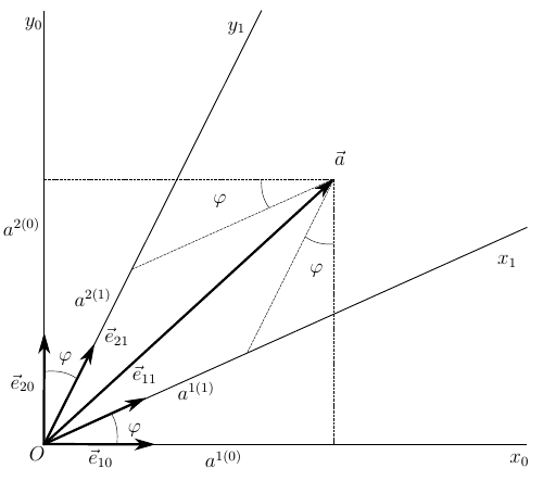
Let the vector given in two normalized bases: rectangular
and oblique . Conversion from an oblique coordinate system to a rectangular one is expressed by a matrix


inverse transform


Let also, in rectangular coordinates, our vector has components


and it is not difficult to see that its length . The metric tensor in an orthonormal basis is represented by the identity matrix


means


Set the angle of the axes and calculate the contravariant components of the vector in oblique axes


Together with the vector, it is necessary to transform the metric tensor


Well, now calculate the length of the vector in the new basis


i.e


and the scalar product and the length of the vector are invariant , that is, unchanged when the coordinates are transformed, as it should be. At the same time, we used essentially the same relation (20) for work in different bases, having previously transformed the metric tensor in accordance with the rule of transformation of vectors in the spaces under consideration
(25).

Conclusion and conclusions

What did we see in the previous paragraph? If the properties of the space in which the vectors are given are known, then it is not difficult for us to perform, in a strictly formal way, actions on the vectors using relations, the form of which is independent of the form of the space. Moreover, relations (20), (24) and (25) give us both an algorithm for calculating and a way of transforming the components of the expressions used by the algorithm. This is the power and strength of the tensor approach.

Many physical theories, such as GR, operate on a curved space-time, and there another approach is simply unacceptable. In the curved space-time, the metric tensor is given locally, at each point, and if we try to do without tensors, nothing will work out for us - we will get cumbersome and cumbersome equations, if we get them at all.

In applied fields of science, the tensor notation of expressions is applicable where it is required to obtain equations independent of the used coordinate system.

But that is not all. We did not talk about the properties of the metric tensor, did not consider the vector product and Levi-Chevita tensor. They did not talk about the rank of the tensors and operations with them, did not fully understand the rules of indexation of the components of tensors and about many other things. This will be written a little later, but for now - thanks to all my readers for their attention.

To be continued...