Skin Detection in Wolfram Language (Mathematica)

Translation of the post by Matthias Odisio " Seeing Skin with Mathematica ".
Download the file containing the text of the article, interactive models and all the code given in the article here .
I express my deep gratitude to Kirill Guzenko for his help in translating.

---

Skin detection can be quite useful - this is one of the main steps to more advanced systems aimed at detecting people, recognizing gestures, faces, filtering based on content, and more. Despite all of the above, my motivation for creating the application was different. The development and research department at Wolfram Research, where I work, has undergone a slight reorganization. With my colleagues who are involved in probabilities and statistics, who have become much closer to me, I decided to develop a small application that would use both the image processing functionality in Mathematica and the statistical functions. Skin detection is the first thing that came to my mind.

Skin shades and appearance may vary, which complicates the task of detection. The detector I wanted to develop is based on probabilistic models for pixel colors. For each pixel of the image applied to the input, a skin detector indicates the probability that this pixel belongs to a skin area.



Let's look at this problem from the point of view of probability theory. We would like to estimate the probability that a pixel belongs to an area with skin of a given color. Using the Bayes formula, we can express it like this (let's call it equation 1):
')


Please note that in this post the probabilities are denoted by the capital P [.].

The three conditions on the right side of the equation can be represented in a computable form. Here the probabilistic approach will be useful to us and these two training data sets: the first consists of pixels belonging to areas with skin, and the second from pixels that do not belong. We will teach a statistical model and get a formula for P [color | skin] . The estimation of a priori P [skin] can be arbitrary in the sense that it depends on the final application for which the skin detector is being developed. We will go in a simple way and determine the prior probability through the ratio of the number of pixels from the two training data sets. With P [color] , there will be more problems at first, because reliable probability modeling for each possible color will require a huge training data set. Fortunately, the full probability formula allows us to circumvent this problem by decomposing this term as follows:



Finally, our probabilistic skin detector will be implemented by the formula (let's call it equation 2):



Let's now create two sets of images and train our model on them.

I know firsthand that creating such collections is something like art, and requires a lot of effort. However, this time we will not be particularly zealous and will collect instead only with a dozen of the images, which depict the skin. Of course, serious statistically significant models would require hundreds of images and complex skin models.

Using the Graphics menu in Mathematica , I can manually select areas with skin in the image and repeat the process for collections with images - frankly, not the most interesting part of my day:



There is evidence that the standard RGB color space is not the best color space for implementing models with color separation by skin / not skin. Most of the problems can arise from the fact that with different lighting and different facial features the skin looks different.

As you can see, the colors of the skin and everything else (shown in red and green, respectively) do not overlap much in the images in the sample, but at the same time cover most of the three-dimensional RGB space:



Let's experiment with a different color space, where such changes in how the skin looks, are modeled, perhaps, more reliably.

CIE XYZ can be selected as the color space, and the skin color can be presented in two color and one luminance coordinates. To develop models that are more resistant to changes in lighting conditions, we will work only with the color coordinates x and y , defined as x = X / ( X + Y + Z ) and y = Y / ( X + Y + Z ):
The colorConvertxy function gives a two-channel xy image:



The list of xy regions with skin is extracted using the image itself, a mask of skin areas and PixelValuePositions and PixelValue functions . A list of pairs of xy areas of the skinless image can be obtained in exactly the same way.



In the two-dimensional xy color space, the regions with coordinates of skin points for all the training images have a smaller area than in RGB, and the difference between the areas with skin and without less pronounced. In the distributions for the colors of areas with and without skin presented below, the first are in shades of green and the second in shades of red.





Work in a two-dimensional xy color space is promising. Let's go back and present the data-based statistical models for equation 2. For the convenience of the reader, we repeat the formula:



The proportion of skinned pixels among the million pixels of the training data set is about 13%. Let's keep this empirical value in our model for a priori probability P [skin] :





To model the probability density functions P [color | skin] and P [color | nonskin], it comes to mind to use a certain mixture of Gaussian distributions. These distributions may well be suitable for these xy pairs presented above. However, on my laptop, calculations are done a little faster when choosing a model based on distributions with a smooth kernel distributions, which are built using the SmoothKernelDistribution function:





Finally, the probability that a given color in xy corresponds to the skin can be represented through the following function:







How will the presented model work? Let's apply the function to several test images:







Not bad, is it? But with another test image below it turns out interesting - the blurred area on the border between the red T-shirt and the green foliage is incorrectly and accurately defined as leather.





Everything is almost done. In fact, skin detection requires deciding whether a pixel belongs to the skin. To create such a binary image, we could set a threshold for the images we received. However, what threshold to choose? If you choose too high, then the skin pixels may not show up. If you choose too low, then the number of skinless pixels defined as skin will be large. All this leads to the construction and analysis of ROC curves. Yes, it would be great to recreate this functionality with Mathematica , but I believe that this topic deserves more attention. In general, another time, in another post.

In an alternative strategy, it is proposed to compare the probabilities for a pixel to be part of an area with skin or not. Like last time, let's use the probabilistic approach and reconsider equation 1: P [skin | color] == P [color | skin] * P [skin] / P [color] . In the same way, it is possible to express the posterior probability that a given pixel does not belong to an area with skin:



To sort this color by skin / not skin, we just need to compare the posterior probabilities obtained and select a large one. P [color] can be dropped, and then the pixel will be defined as belonging to the skin area if P [color | skin] * P [skin]> P [color | nonskin] * P [nonskin] .

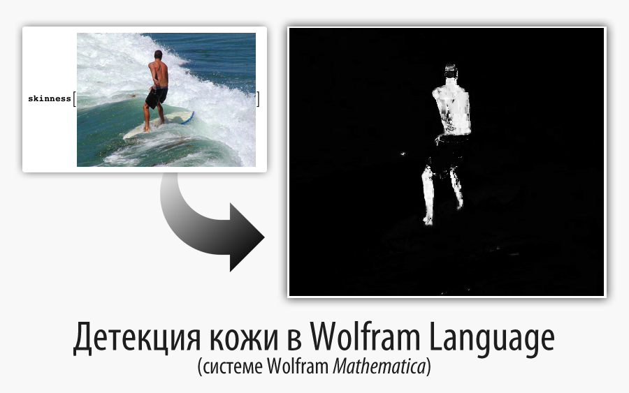
Here is how the skin detector works at the moment:



A quick assessment of test images allows us to conclude that the system copes well with the task:





Let's end this topic with a skin detection application:





Initially, my goal was to create a skin detector purely from pleasure in exploring the interactions between probabilities, statistics, and image processing. Practically every element of our final version of a skin detector (for example, a training sample, a choice of statistical distributions, a classifier, a quantitative assessment) can be studied in more detail and improved using the wide functionality of Mathematica .