5 ways to calculate Fibonacci numbers: implementation and comparison

Introduction

Programmers Fibonacci numbers should already podnadoest. Examples of their calculations are used everywhere. All that these numbers provide the simplest example of recursion. They are also a good example of dynamic programming. But is it necessary to calculate them in a real project? Do not. Neither recursion nor dynamic programming is ideal. And not a closed formula using floating point numbers. Now I will tell you how. But first, let's go through all the known solutions.

The code is intended for Python 3, although it should go in Python 2.

To begin with, let me remind you the definition
')
F _n = F _n-1 + F _n-2

and F ₁ = F ₂ = 1.

Closed formula

Let's skip the details, but those who wish can get acquainted with the derivation of the formula . The idea is to assume that there is some x for which F _n = x ⁿ , and then find x.



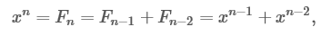
which means



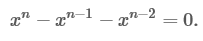
cut x ^n-2



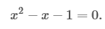
Solve the quadratic equation:



From where the “golden ratio” ϕ = (1 + √5) / 2 grows. Substituting the original values ​​and doing another calculation, we get:



which we use to calculate F _n .

from __future__ import division import math def fib(n): SQRT5 = math.sqrt(5) PHI = (SQRT5 + 1) / 2 return int(PHI ** n / SQRT5 + 0.5) 

Good:
Fast and easy for small n
The bad:
Requires floating point operations. For large n, greater accuracy is required.
Evil:
Using complex numbers to calculate F _{n is} beautiful from a mathematical point of view, but ugly from a computer.

Recursion

The most obvious solution that you have already seen many times is most likely as an example of what recursion is. I repeat it again, for completeness. In Python, it can be written in one line:

 fib = lambda n: fib(n - 1) + fib(n - 2) if n > 2 else 1 

Good:
Very simple implementation, repeating the mathematical definition
The bad:
Exponential lead time. For large n very slowly
Evil:
Stack overflow

Memorization

The recursion solution has a big problem: overlapping calculations. When fib (n) is called, fib (n-1) and fib (n-2) are counted. But when fib (n-1) is considered, it again independently calculates fib (n-2) —that is, fib (n-2) is counted twice. If we continue the argument, it will be seen that fib (n-3) will be counted three times, and so on. Too many intersections.

Therefore, you just need to memorize the results so as not to count them again. Time and memory of this solution are spent in a linear fashion. I use a dictionary in the solution, but I could use a simple array.

 M = {0: 0, 1: 1} def fib(n): if n in M: return M[n] M[n] = fib(n - 1) + fib(n - 2) return M[n] 

(In Python, this can also be done using a decorator, functools.lru_cache.)

Good:
Just turn recursion into a memorized solution. Turns exponential time into linear execution, which consumes more memory.
The bad:
Spends a lot of memory
Evil:
Possible stack overflow, like recursion

Dynamic programming

After solving with memorization, it becomes clear that we do not need all the previous results, but only the last two. In addition, instead of starting with fib (n) and going backwards, you can start with fib (0) and go forward. The following code has linear execution time, and memory usage is fixed. In practice, the solution speed will be even higher, since there are no recursive function calls and related work. And the code looks simpler.

This solution is often cited as an example of dynamic programming.

 def fib(n): a = 0 b = 1 for __ in range(n): a, b = b, a + b return a 

Good:
Fast for small n, simple code
The bad:
Still linear execution time
Evil:
Yes, nothing special.

Matrix algebra

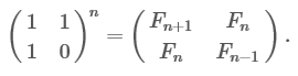
And, finally, the least illuminated, but the most correct solution, competently using both time and memory. It can also be extended to any homogeneous linear sequence. The idea of ​​using matrices. It is enough just to see that



A generalization of this suggests that



Two values ​​for x, obtained by us earlier, one of which was the golden section, are eigenvalues ​​of the matrix. Therefore, another way to derive a closed formula is to use the matrix equation and linear algebra.

So why is such a formulation helpful? The fact that exponentiation can be made in logarithmic time. This is done through squaring . The bottom line is that



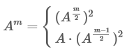
where the first expression is used for even A, the second for odd. It remains only to organize the multiplication of matrices, and everything is ready. It turns out the following code. I organized the recursive implementation of pow, since it is easier to understand. Iterative version, see here.

 def pow(x, n, I, mult): """  x   n. ,  I –   ,    mult,  n –   """ if n == 0: return I elif n == 1: return x else: y = pow(x, n // 2, I, mult) y = mult(y, y) if n % 2: y = mult(x, y) return y def identity_matrix(n): """   n  n""" r = list(range(n)) return [[1 if i == j else 0 for i in r] for j in r] def matrix_multiply(A, B): BT = list(zip(*B)) return [[sum(a * b for a, b in zip(row_a, col_b)) for col_b in BT] for row_a in A] def fib(n): F = pow([[1, 1], [1, 0]], n, identity_matrix(2), matrix_multiply) return F[0][1] 

Good:
Fixed memory, logarithmic time
The bad:
The code is more complicated
Evil:
We have to work with matrices, although they are not so bad

Performance comparison

It is worth comparing only the variant of dynamic programming and the matrix. If we compare them by the number of characters in the number n, then it turns out that the matrix solution is linear, and the solution with dynamic programming is exponential. A practical example is the calculation of fib (10 ** 6), a number that has more than two hundred thousand characters.

n = 10 ** 6
We calculate fib_matrix: fib (n) has only 208988 digits, the calculation took 0.24993 seconds.
We calculate fib_dynamic: fib (n) has only 208988 digits, the calculation took 11.83377 seconds.

---

Theoretical notes

Without directly relating to the above code, this comment still has a certain interest. Consider the following graph:



Let us calculate the number of paths of length n from A to B. For example, for n = 1 we have one path, 1. For n = 2, we again have one path, 01. For n = 3, we have two paths, 001 and 101 Quite simply, it can be shown that the number of paths of length n from A to B is exactly F _n . Writing the adjacency matrix for the graph, we get the same matrix that was described above. This is a well-known result from graph theory that, for a given adjacency matrix A, occurrences in A ⁿ are the number of paths of length n in the graph ( one of the problems mentioned in the film "Good Will Hunting").

Why are there such symbols on the edges? It turns out that if you consider an infinite sequence of characters on an infinite sequence of paths on both sides of a graph, you will get something called “ finite type poddvigi ”, which is a type of system of symbolic dynamics. Specifically, this finite type subdivision is known as the “golden section shift”, and is defined by the set of “forbidden words” {11}. In other words, we get infinite in both directions binary sequences and no pairs of them will be adjacent. The topological entropy of this dynamical system is equal to the golden section ϕ. I wonder how this number periodically appears in different areas of mathematics.