Search for quadrangle documents on mobile devices

Some of the document recognition modules developed by our company, as the first stage of their work, should determine the location of the object on the incoming image or in the video stream. Today’s article is devoted to one of our approaches to solving this problem.

Formulation of the problem

To begin with, we will determine what information we can use for our own purposes.
In applications, the intended types of documents are sufficiently rigid. We assume that no one is seriously trying to recognize a passport as an application for bank cards or vice versa, which means that we know, at least, the proportions of the desired object. Also note that the absolute majority of mobile devices have cameras with a fixed focal length.

Since the found has yet to be recognized, it makes sense to look at far from any image of the document. In order not to get a photo at the entrance with a small piece of the document in the corner of the diagonals, we use some restrictions and accompany them with visualization, which would help the user to get a suitable frame layout at the shooting stage.
Specifically, I would like to meet the following conditions:
1 - recognizable document must be entirely in the frame.
2 - the document should occupy a large enough part of the frame.
')
To achieve the fulfillment of these conditions can be different. If you directly demand that the document occupy no less than X% of the frame area, you can hear the well-grounded grinding of user's teeth, since it’s very difficult to see if the document occupies, say, 80% of the frame area, or only 75%.
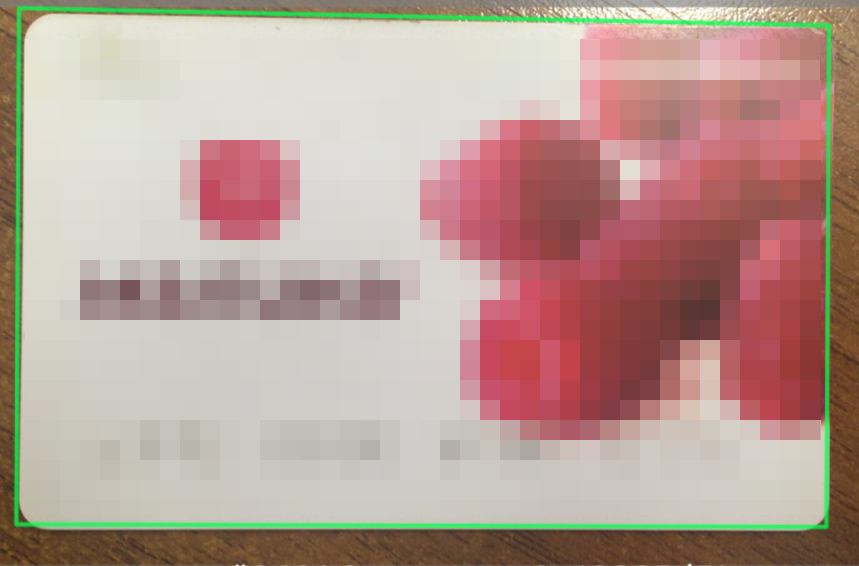
But there are much more visual options. So, you can set the permissible rectangular zones for each of the vertices of the document border and suggest the user to direct the camera in such a way that each side of the document completely lies on one side of the document.

For the user, this might look like this:


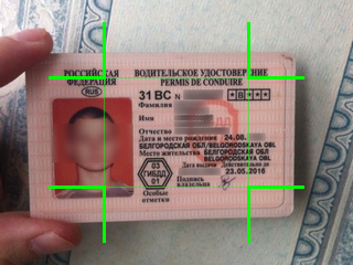
In addition to visualization for the user, this method imposes an additional useful limitation on the position of the document: based on the size of the zones, you can calculate the maximum possible angles of inclination of the sides to the axes, and, as a result, the range of possible deviations of the quadrilateral angles from 90 degrees. Well, or, conversely, it is possible to set such zone sizes so that the deviations of these parameters do not exceed certain threshold values.

From this point on, one can observe maneuvering between Scylla and Charybdis of any image processing algorithm — speed and accuracy / quality of work.

Highlighting borders

First of all, we will reduce the input image to a smaller size in order to reduce the time costs. We use a cast to 320px on the larger side as some optimum selected for specific user cases.
To search for a document, we will only need image regions corresponding to 4 side zones. In each of them we will look for borders that could be the edges of the document.
Further manipulations will be considered on the example of the upper region - for the rest, the actions are similar up to a rotation of 90 degrees (*).

1. Calculate the image gradient by suppressing high-frequency noise using a Gaussian filter. Due to restrictions on the location of the document, we are only interested in orthotropic boundaries, i.e. directed mainly along one of the coordinate axes (in the case of the upper region, along the axis OX). To search for such boundaries, the derivative along the OY axis is sufficient. The problem is that the color image is a vector image, and its derivative is also a vector, but in the one-dimensional case, to estimate the severity of the border, we can take some norm of this vector, unlike the full gradient, which is much more complicated to calculate, for example, by Di Zenzo [ one].
   To avoid unnecessary arithmetic operations, we use norm, i.e. take the derivative module in each channel
   
   
   
   
   and then choose the largest of these values
   
   
   
   
   resulting in a halftone image derivative.
   
2. We filter the resulting image: first we use the classical non-maximum suppression (see Canny [2]) and get the initial map of boundaries, then suppress the outliers generated by the textures. To do this, multiply the value of each pixel G (x, y) of the borders by the following coefficient k:
   
   
   
   
   where ht is the height of the region, and for ₀ , y ₁ are the y-coordinates of the closest to the current boundary pixels above and below, or the fake values ​​if there are none.
   
3. We collect the boundary pixels into connected components — they have more possible clipping parameters than individual pixels. In our implementation, components whose size or average brightness is less than the threshold values ​​are discarded.
   

* The search for boundaries (and then direct) in each region occurs independently of the others, which means it is perfectly parallelized.

Search direct

The next step is to extract the lines using the fast Hough transform [3] (*). The Hough transformation translates the boundary map into a battery matrix, each cell (i, j) of which corresponds to a parametrically defined straight line, and local maxima in such a battery correspond to the most significant straight lines on the boundary map.
In many cases, the best direct one is not enough - the restrictions will not protect us from a table / keyboard / keyboard / anything else that is longer and more contrast than our document. However, a cunning plan to simply take some of the largest values ​​in a battery is doomed to failure: each straight line actually forms some maximum neighborhood in the battery (see figure below), and the first few maxima most likely will correspond to approximately the same straight line.
Since our goal is not to find out with great precision the location of one straight line, but to dial several quite different ones, this does not suit us.
Therefore, the following iterative procedure takes place in the combat version of the algorithm:

1. Transformation of Hafa over the boundary map
2. Adding the best direct to the answer
3. If the number of lines is less than the required - rubbing the found straight line on the map of boundaries and return to point 1

Each of the received direct we will supply with weight - value from the corresponding cell of the accumulator Hough.

* By fast Hough transform, we mean an exact fast implementation, not an approximation of a transform.

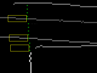
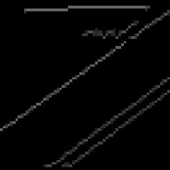a) border map	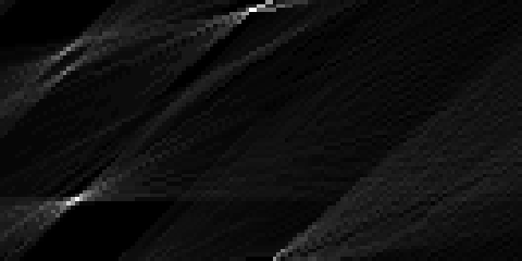b) BPH battery
An example of the operation of BPH. (Did you understand which of the straight lines corresponds to each of the peaks on the battery?)

Combinatorial scheme

After the previous step, we have 4 sets of lines - one for each side of the document. From these direct combinatorial enumeration we compose all possible quadrilaterals, among which we will search for the most plausible. As an initial estimate C of each of the quadrangles, we take the sum of the weights of the lines from which it is assembled. All subsequent steps are devoted to the adjustment of this assessment, taking into account the emergent characteristics of the quadrilateral.

If the lines in the neighboring areas do not break at the point of their intersection, but continue beyond it, then it is highly likely that this is not the angle of the desired object, but something else. Of course, there may be a case where the border of the document is located along a certain direct background, and, moreover, even at a real angle several pixels can crawl away during image processing, but in general this is a bad sign. Such “getting out” of lines for a corner will be fined:


where p _i is the penalty for the i-th angle, which is the sum of the intensities of the first n pixels on the boundary map behind the intersection point along the straight lines forming the angle.
->
An example for the upper left corner. Yellow denotes the penalty area for horizontal lines.

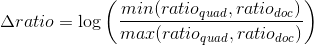
Further, using the focal distance known to us, for each of the quadrangles we reconstruct the parallelogram [4] (the only one up to homothety) whose projective image is this quadrilateral. Let us compare the aspect ratio of the obtained parallelogram with the known aspect ratio of the desired document, and its angles - with the right angles, which the document, like, should have. For the deviation of these parameters from the expected also introduce penalties:



Then if :



where A, B, α, β - optimized coefficients,
T _a , T _r - threshold values.

That's all. The quad with the greatest weight is taken for the location of the document on the image.

results

The test sample for quality assessment consists of 6000 photographs of documents on a different background and 6000 regular quadrangles, respectively. The initial resolution of images varies from 640x480 to 800x600. The test device is an iPhone 4S (photos were taken from it and shrunk to the specified permissions from the outside of the described algorithm).

To assess the accuracy of finding the document, the following error function was used:


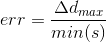
where ∆d _max - the maximum of the distances between the corresponding angles of the true and found quadrangles,
min (s) is the length of the minimal side of a true quadrilateral.

It has been empirically found out that for sufficiently good character recognition on a detected document with side zones occupying 30% of the corresponding size, the value of err should be less than 0.06.

The overall quality of the algorithm was calculated as


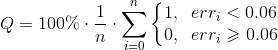
According to this estimate, on a test sample of 6000 images, the quadrangles of documents are at a quality of 98.5%.

The average running time of the algorithm on iPhone 4S is 0.043s (23.2FPS), of which:
scaling - 0.014s,
search for edges - 0.023s,
direct search - 0.005s,
bust with clipping - 0.001s.

Literature

[1] S. Di Zenzo. A note on the gradient of a multi-image.
[2] J. Canny. A computational approach to edge detection.
[3] DP Nikolaev et al. Hough transform: underestimated tool in computer vision field.
[4] Z. Zhang. Whiteboard scanning and image enhancement.