"Big battalions" in continuous time (battle simulation)
"God is always on the side of the big battalions" - Jacques d'Estamp de Ferté, French marshal
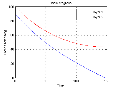 Fig. one
Many computer games need to simulate battles without displaying their progress on the screen. For example, it could be a Rogue-like turn-based game in which the computer should count only the outcome of the battle (who won) and the loss of the parties. Even in interactive games, battles that occur outside of the player’s field of view can be modeled oversimplified. I developed an interesting mathematical model for such modeling and present it to readers.
')
The article discusses the "continuous" approach - that is, the forces of the parties are continuous quantities, and their interaction occurs in continuous time. This allows you to use the methods of the mat. analysis and get the solution explicitly. For armies consisting of a large number of combat units, such a simplification does not introduce a large margin of error. At the same time, the solution explicitly allows us to understand a lot about the problem.
Baseline data for battle simulation is usually the strength of the parties — the number of soldiers or other combat units. There are cases of heterogeneous armies consisting of several types of combat units. But for the time being we will leave these difficulties aside and consider the simplest case: the meeting of two armies consisting of identical soldiers, in equal combat conditions, and differing only quantitatively.
Therefore, the initial data we will have two numbers - the number of soldiers in each army at the time of the start of the battle.
In real battles, soldiers shoot at each other or attack in melee. Each act of attack is discrete, the attack can lead to the defeat of the enemy or pass by. After the attack, the soldier must reload or refocus his gun, or wipe the sword again, i.e. one way or another, he may not make another attack right away. The effectiveness of attacks depends on the power of the soldier’s weapons, the strength of the enemy’s armor, the agility of both, and other factors. But all these difficulties without much damage to the accuracy of modeling can be replaced by one factor.
Let k be a coefficient that determines how many opponents on average kill each soldier per unit of time. Practically everything can be taken into account in this coefficient: the improvement of a weapon or accuracy increases k; armor and dodge of the enemy - reduce; You can also take into account the influence of the terrain on the battlefield, time of day, etc.
It rarely happens that armies consist of completely similar soldiers and are found in absolutely equal conditions. "The defense is stronger than the offensive" (R. Clausewitz). Therefore, the coefficient k for each army will be different. But we will not complicate it yet and assume that the coefficient k is the same for both armies, and later we will generalize the results to the case of different coefficients.
Let x (t) be the number of soldiers of the first army, which decreases as the enemy kills them. Let y (t) be the number of soldiers of the second army. Then the interaction model described above can literally be literally translated into a mathematical language:

That is: the rate of loss of soldiers of the first army is proportional to the number of soldiers in the second army, and vice versa.
The result was a system of differential equations. It is easily solved, in particular, with the help of Wolfram Alpha. Common decision:
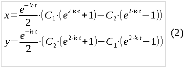
Where C1 and C2 are the integration constants that must be found on the basis of the initial conditions. If the number of soldiers of the first army at the start of the battle t = 0 is x0, and the second army, respectively, y0 - then we substitute and get C1 = x0, C2 = y. After simplification, the particular solution we need finally looks like this:
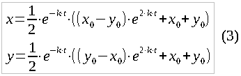
So, we found functions that establish the dependence of the number of remaining soldiers of each of the parties on the time spent in the battle. An example of the graph of such functions is shown in Fig. one.
What behavior can be expected from the functions obtained?
For example, we substitute x0 = y0, i.e. we will model the battle between equal armies and see what happens. The term c exp (2 * k * t) is destroyed, and x (t) = y (t) = x0 * exp (-k * t) remains. Both armies destroy each other exponentially, their numbers decrease very quickly, but they never reach zero. The battle will last forever, and the infinitesimal number of the remaining soldiers will be compensated by the infinitesimal speed of their loss.
If we now substitute different values, for example, x0 = 90 and y0 = 100 (as in Fig. 1), then the term with exp (2 * k * t) will act differently for each army. That army, which initially had more soldiers, will receive a "supplement" from exp (2 * k * t) in a positive direction, that is, its speed of decline will slow down. The other army, smaller, will receive the same “additive” in the minus, so that it will thin out faster. As a result, in a finite time t1, the number of the weaker army will reach zero. The battle will end with the defeat of this army.
Look at pic again. 1. It can be seen that at the beginning of the graph, both functions decrease approximately equally, since the difference in the number of armies is small. But gradually the difference in the rate of decline increases, and this is a self-sustaining effect. A small initial numerical advantage (only 10%) not only ensures victory in the battle, but almost half of the soldiers of the victorious army survive.
The result is all the more impressive that the graph in fig. 1 was built based on the value of k = 0.01. Imagine that time is measured in minutes. This means that every minute an army soldier kills an average of 0.01 enemy soldiers. That is, for example, he shoots every minute once, and hits with a probability of 1%. This is a very low rate of fire and the probability of hitting. However, the battle ends in about 150 minutes with the complete destruction of a weaker army. This is all due to the fact that we have exhibitors in the solutions.
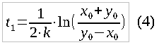
Calculating x (t) and y (t) after one of these functions has reached zero (that is, after the victory of one of the parties) makes no sense. So, in particular, when t> t1, x (t) will become less than zero, and y (t) will start to grow. To know to what value of t to conduct calculations, one should find t1.
Let us find the moment of the defeat of t1 for the case of x0 <y0. Substitute x (t1) = 0 into formula (3) and after transformations we get:
Now you can bring Matlab-code, which uses formulas (3) and (4) to plot the course of the battle.
It is also of interest to find the loss of the winning side. Substituting the found t1 from formula (4) into formula (3), after transformations, we get:
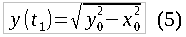
In principle, formula (5) is the main result of this article, as it was already clear that the larger army wins, and if we are not interested in the course of the battle, but only its result, then it is necessary to find only the losses of the winning party.
It is curious that the losses of the winner do not depend on k, but depend only on the initial balance of forces. Only the duration of the battle depends on k.
Let us try to express the time of the battle and the loss of the winner not through the absolute values x0 and y0, but through their ratio. Let r = x0 / y0 (0 <r <1 for x0 <y0), then x0 = r * y0 and after transformations we get:

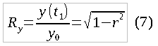
Losses of the winner will be found as the ratio of the number of soldiers after the battle to the number of soldiers before the battle:
In fig. 2 shows a graph of the function Ry (r):
 Fig. 2
It can be seen that the victorious army suffers small losses in general, which confirms the thesis on large battalions in the epigraph. Even with a 10: 9 aspect ratio, almost half of the victorious army survive, and only when r> 0.95, the winner has significant losses, which can be said about “Pyrrhic Pobda”.
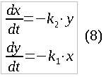
Unequal combat conditions (differences in training of soldiers, armaments, armor, defense against offensive, terrain factors) can be taken into account if different coefficients k1 and k2 are introduced in the system of equations (1) instead of one k. That is, the average rate of extermination of the enemy from the soldiers of each of the armies will differ:
The particular solution of such a system we need, similar to formula (3), looks like this:
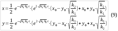
The expressions were more cumbersome, but if we introduce the substitution: p = sqrt (k1 * k2), r = sqrt (k1 / k2) * x0 / y0 - then everything is greatly simplified:

In principle, if we make a similar substitution for system (3), then systems (3) and (10) will look the same, and the difference between them will be only in the expression for r: for the case of different k1 and k2, the multiplier appears in the expression for r sqrt type (k1 / k2).
The victory criterion is now a comparison of r with 1. If r> 1, then the first army (x) wins, if r <1, then the second (y). With r = 1, both armies are mutually destroyed in infinite time.
The time of victory coincides with formula (6) with the only difference that instead of k now p appears:

And finally, the remaining soldiers of the winner: the formula (7) is applicable without changes in the case of using a new substitution for r.
Simulating battles in continuous functions allows you to get reasonable results with minimal computational overhead. Even in the more complicated case of unequal battle conditions, the result of the battle can be calculated with just three calls of a square root and several additions, multiplications and divisions. Computational complexity - O (1).
The advantage of the "big battalions" very clearly follows from the above formulas and graphs. Particularly impressive is the fact that even a small numerical advantage in the model leads to the complete defeat of the enemy with much smaller losses than can be intuitively expected.
Why is the outcome of real battles so unpredictable, unlike the model? Of course, due to the influence of random factors that are unknown during the calculations. In my model, the effect of randomness can be reflected somewhere in the coefficients k1 and k2. These coefficients in a decisive way influence the outcome of the battle and can outweigh the balance in one direction or another.
The approach proposed by me can be developed in that direction in order to apply a theorem and a mat to it. statistics. It would also be interesting to develop a model for heterogeneous armies consisting of several types of troops. But this is a topic for individual research and a new article. Thanks for attention.
Fig. oneMany computer games need to simulate battles without displaying their progress on the screen. For example, it could be a Rogue-like turn-based game in which the computer should count only the outcome of the battle (who won) and the loss of the parties. Even in interactive games, battles that occur outside of the player’s field of view can be modeled oversimplified. I developed an interesting mathematical model for such modeling and present it to readers.
')
The article discusses the "continuous" approach - that is, the forces of the parties are continuous quantities, and their interaction occurs in continuous time. This allows you to use the methods of the mat. analysis and get the solution explicitly. For armies consisting of a large number of combat units, such a simplification does not introduce a large margin of error. At the same time, the solution explicitly allows us to understand a lot about the problem.
Initial data
Baseline data for battle simulation is usually the strength of the parties — the number of soldiers or other combat units. There are cases of heterogeneous armies consisting of several types of combat units. But for the time being we will leave these difficulties aside and consider the simplest case: the meeting of two armies consisting of identical soldiers, in equal combat conditions, and differing only quantitatively.
Therefore, the initial data we will have two numbers - the number of soldiers in each army at the time of the start of the battle.
Interaction model
In real battles, soldiers shoot at each other or attack in melee. Each act of attack is discrete, the attack can lead to the defeat of the enemy or pass by. After the attack, the soldier must reload or refocus his gun, or wipe the sword again, i.e. one way or another, he may not make another attack right away. The effectiveness of attacks depends on the power of the soldier’s weapons, the strength of the enemy’s armor, the agility of both, and other factors. But all these difficulties without much damage to the accuracy of modeling can be replaced by one factor.
Let k be a coefficient that determines how many opponents on average kill each soldier per unit of time. Practically everything can be taken into account in this coefficient: the improvement of a weapon or accuracy increases k; armor and dodge of the enemy - reduce; You can also take into account the influence of the terrain on the battlefield, time of day, etc.
It rarely happens that armies consist of completely similar soldiers and are found in absolutely equal conditions. "The defense is stronger than the offensive" (R. Clausewitz). Therefore, the coefficient k for each army will be different. But we will not complicate it yet and assume that the coefficient k is the same for both armies, and later we will generalize the results to the case of different coefficients.
Basic equations and their solution
Let x (t) be the number of soldiers of the first army, which decreases as the enemy kills them. Let y (t) be the number of soldiers of the second army. Then the interaction model described above can literally be literally translated into a mathematical language:
That is: the rate of loss of soldiers of the first army is proportional to the number of soldiers in the second army, and vice versa.
The result was a system of differential equations. It is easily solved, in particular, with the help of Wolfram Alpha. Common decision:
Where C1 and C2 are the integration constants that must be found on the basis of the initial conditions. If the number of soldiers of the first army at the start of the battle t = 0 is x0, and the second army, respectively, y0 - then we substitute and get C1 = x0, C2 = y. After simplification, the particular solution we need finally looks like this:
So, we found functions that establish the dependence of the number of remaining soldiers of each of the parties on the time spent in the battle. An example of the graph of such functions is shown in Fig. one.
Results analysis
What behavior can be expected from the functions obtained?
For example, we substitute x0 = y0, i.e. we will model the battle between equal armies and see what happens. The term c exp (2 * k * t) is destroyed, and x (t) = y (t) = x0 * exp (-k * t) remains. Both armies destroy each other exponentially, their numbers decrease very quickly, but they never reach zero. The battle will last forever, and the infinitesimal number of the remaining soldiers will be compensated by the infinitesimal speed of their loss.
If we now substitute different values, for example, x0 = 90 and y0 = 100 (as in Fig. 1), then the term with exp (2 * k * t) will act differently for each army. That army, which initially had more soldiers, will receive a "supplement" from exp (2 * k * t) in a positive direction, that is, its speed of decline will slow down. The other army, smaller, will receive the same “additive” in the minus, so that it will thin out faster. As a result, in a finite time t1, the number of the weaker army will reach zero. The battle will end with the defeat of this army.
Look at pic again. 1. It can be seen that at the beginning of the graph, both functions decrease approximately equally, since the difference in the number of armies is small. But gradually the difference in the rate of decline increases, and this is a self-sustaining effect. A small initial numerical advantage (only 10%) not only ensures victory in the battle, but almost half of the soldiers of the victorious army survive.
The result is all the more impressive that the graph in fig. 1 was built based on the value of k = 0.01. Imagine that time is measured in minutes. This means that every minute an army soldier kills an average of 0.01 enemy soldiers. That is, for example, he shoots every minute once, and hits with a probability of 1%. This is a very low rate of fire and the probability of hitting. However, the battle ends in about 150 minutes with the complete destruction of a weaker army. This is all due to the fact that we have exhibitors in the solutions.
Calculating x (t) and y (t) after one of these functions has reached zero (that is, after the victory of one of the parties) makes no sense. So, in particular, when t> t1, x (t) will become less than zero, and y (t) will start to grow. To know to what value of t to conduct calculations, one should find t1.
Derivation of formulas for the victory time t1 and the losses of the winning army
Let us find the moment of the defeat of t1 for the case of x0 <y0. Substitute x (t1) = 0 into formula (3) and after transformations we get:
Now you can bring Matlab-code, which uses formulas (3) and (4) to plot the course of the battle.
Drawing drawing program for fig. one
x0 = 90; % Number of soldiers in army-1 y0 = 100; % Number of soldiers in army-2 k = 0.01; % Damage to armor factor %---------------------------------- if x0~=y0 t_end = log((x0+y0)./abs(x0-y0))./2./k; else t_end = 1000; end t = [0:floor(t_end) t_end]; x = 0.5*exp(-k*t).*((x0-y0)*exp(2*k*t)+x0+y0); y = 0.5*exp(-k*t).*((y0-x0)*exp(2*k*t)+x0+y0); figure(1); plot(t,x); hold on plot(t,y,'r'); hold off grid on ylim([0 max(x0,y0)]); xlabel('Time') ylabel('Forces remaining') legend({'Player 1','Player 2'}) title('Battle progress') It is also of interest to find the loss of the winning side. Substituting the found t1 from formula (4) into formula (3), after transformations, we get:
In principle, formula (5) is the main result of this article, as it was already clear that the larger army wins, and if we are not interested in the course of the battle, but only its result, then it is necessary to find only the losses of the winning party.
It is curious that the losses of the winner do not depend on k, but depend only on the initial balance of forces. Only the duration of the battle depends on k.
Let us try to express the time of the battle and the loss of the winner not through the absolute values x0 and y0, but through their ratio. Let r = x0 / y0 (0 <r <1 for x0 <y0), then x0 = r * y0 and after transformations we get:
Losses of the winner will be found as the ratio of the number of soldiers after the battle to the number of soldiers before the battle:
In fig. 2 shows a graph of the function Ry (r):
Fig. 2It can be seen that the victorious army suffers small losses in general, which confirms the thesis on large battalions in the epigraph. Even with a 10: 9 aspect ratio, almost half of the victorious army survive, and only when r> 0.95, the winner has significant losses, which can be said about “Pyrrhic Pobda”.
Generalization in case of unequal combat conditions
Unequal combat conditions (differences in training of soldiers, armaments, armor, defense against offensive, terrain factors) can be taken into account if different coefficients k1 and k2 are introduced in the system of equations (1) instead of one k. That is, the average rate of extermination of the enemy from the soldiers of each of the armies will differ:
The particular solution of such a system we need, similar to formula (3), looks like this:
The expressions were more cumbersome, but if we introduce the substitution: p = sqrt (k1 * k2), r = sqrt (k1 / k2) * x0 / y0 - then everything is greatly simplified:
In principle, if we make a similar substitution for system (3), then systems (3) and (10) will look the same, and the difference between them will be only in the expression for r: for the case of different k1 and k2, the multiplier appears in the expression for r sqrt type (k1 / k2).
The victory criterion is now a comparison of r with 1. If r> 1, then the first army (x) wins, if r <1, then the second (y). With r = 1, both armies are mutually destroyed in infinite time.
The time of victory coincides with formula (6) with the only difference that instead of k now p appears:
And finally, the remaining soldiers of the winner: the formula (7) is applicable without changes in the case of using a new substitution for r.
Conclusion
Simulating battles in continuous functions allows you to get reasonable results with minimal computational overhead. Even in the more complicated case of unequal battle conditions, the result of the battle can be calculated with just three calls of a square root and several additions, multiplications and divisions. Computational complexity - O (1).
The advantage of the "big battalions" very clearly follows from the above formulas and graphs. Particularly impressive is the fact that even a small numerical advantage in the model leads to the complete defeat of the enemy with much smaller losses than can be intuitively expected.
Why is the outcome of real battles so unpredictable, unlike the model? Of course, due to the influence of random factors that are unknown during the calculations. In my model, the effect of randomness can be reflected somewhere in the coefficients k1 and k2. These coefficients in a decisive way influence the outcome of the battle and can outweigh the balance in one direction or another.
The approach proposed by me can be developed in that direction in order to apply a theorem and a mat to it. statistics. It would also be interesting to develop a model for heterogeneous armies consisting of several types of troops. But this is a topic for individual research and a new article. Thanks for attention.
Source: https://habr.com/ru/post/260255/
All Articles