Virtual Time Part 2: Simulation and Virtualization Issues
In the previous article, I reviewed the time sources in the PC platform, their features, shortcomings, and history. Now, armed with this knowledge, we can consider how these devices can be represented inside a virtual environment - a full-platform software simulator or a system virtual machine, i.e. software environment that allows you to run inside the operating system.
In this article, we will examine various ways of representing time within models, approaches to simulating the work of timers, the possibility of hardware acceleration during virtualization, and the difficulties of coordinating the flow of time within simulated environments.
Simulators and virtual machines will include software such as Bochs, KVM / Qemu, VMware ESX, Oracle Virtualbox, Wind River Simics, Microsoft HyperV, etc. They allow you to load unmodified operating systems inside you. Accordingly, inside the computer model there should be models of individual devices: processors, memory, expansion cards, input / output devices, etc., as well as, of course, watches, stopwatches and alarms.
')
As in the previous article, we begin the discussion with the requirements for the concept of “time” inside simulators and virtual machines.
Two important properties of the "correct" simulation.
1. Representation of the state of a certain real system and its components with a certain chosen accuracy . The flow of time in the model can be approximate and quite different from reality.
2. Permissible in reality evolution of the state inside the model.
For this, the iron should work a causal relationship . With the exception, perhaps, of some completely exotic systems, the evolution of the system being modeled must correctly order the related events. Those who wish to further explore this very difficult question will recommend starting with the work of Leslie Lamport [2] or similar articles on distributed algorithms.
This may seem strange, but the other conditions for virtual time are not as universal; however, consider them.
The condition of strict monotony of the flow of time. Most often, the virtual time should not decrease with the passage of physical time. As my experience has shown, the “we will reduce time for a minute” approach usually leads to terrible confusion when debugging and is a sign of poor design.
In a number of not quite typical, but still practically important cases, virtual time must move backwards: when the state of optimistic parallel models rolls back , or when it is reversed .
Finally, complex computer systems (and their models) are distributed. For them, the requirement of a common common clock can be excessively strict - parts of such a system should be able to work normally, having only limited local information about time. In them, global time becomes a “vector” quantity. As you know, the vectors are quite difficult to compare on the principle of "more-less."
The condition that the simulated time matches the real time is often redundant. As my practice has shown, to imply any correlation between them is harmful for the simulator's designer, since this creates unreasonable expectations and prevents from creating a correct or fast model. The simplest example: a virtual machine can always be paused; at the same time, the time inside it will stop, we are unable to stop the real time so far.
More interesting example. When the simulation is running, the rate of change of the simulated time can change dynamically. It can be both slower than the real, and much faster. In fact, the simulator often performs programmatically (spending more time on it) what is actually done in hardware. The opposite situation is possible, for example, when the guest system itself is much more “slower” than the host: by simulating a 1 MHz microcontroller on a 3 GHz microprocessor, it is quite possible to drive the code of its firmware ten times faster than reality. Another example: if the simulator detects the inaction of a simulated system (waiting for resources or input, energy-saving mode), then it can advance its time abruptly, thereby outperforming reality (see “event-driven simulation” below).
An important special case: if a simulation implies an interactive interaction with a person with it or, for example, a network interaction, then too high a speed is contraindicated. Life example: the login prompt on Unix-systems first asks for a name, and then a password. If after entering the name the program does not receive the password for some time, it returns to the login (apparently, this is a security measure for cases if the user was distracted by entering the password). When simulating, the virtual time between entering a name and waiting for a password can fly very quickly, in a fraction of a real second - because the guest is idle! As a result, the unfortunate person does not have time to log in to the VM either on the first attempt or on the fifth. In order to completely ruin his life, after three seconds the screen of the simulated system turns black - the screen saver is turned on, because an hour has passed for the guest system in idleness!
Of course, this is easily treated by introducing a “real-time mode”, when the simulator itself pauses in its work, thereby slowing down the passage of time in the guest to an average value of “second per second.”
In the opposite direction, alas, it does not work. If at some computationally complicated part of the guest’s work the simulator manages to advance the virtual time by just a few milliseconds in one real second, the user will notice: “FPS has fallen”. To compensate for this by reducing the level of detail, most likely, it will not work: you cannot throw off the start of processes from the OS loading, you cannot omit a part of the algorithm from the archiver program.
The first idea that comes to mind when it is necessary to simulate the flow of a process: choose a sufficiently small interval for the basic indivisible unit of time. Then promote virtual time in such small steps, at each one simulating all changes in the system that have occurred over the elapsed time interval. The idea of this method is from thecourse of practice of modeling analog processes and continuous in time functions on discrete computers.
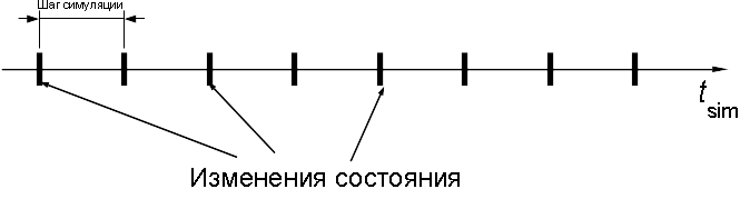
This type of simulation with a fixed pitch (English time-stepped simulation) is quite simple and most harmoniously combined with scenarios, when there are really some events at each simulation step. For example, this is true for the in-camera models of digital devices — when modeling the CPU pipeline and associated nodes. In reality, on each front of the clock signal, the state of the registers, queues, and counters change. Such a model can be generated by tools accepting input descriptions in hardware design languages such as SystemVerilog or VHDL.
However, in higher-level models, such as functional simulators and virtual machines, the situation with events is somewhat different. Such programs operate with models of whole devices (timers, disks, network cards, etc.) and transactions between them. It is transactions, rather than internal processes, that cause most of the changes in the states of such a system (to simulate which is the primary task of the simulator), and at the same time they are asynchronous and not tied to any measure with a fixed length. A fixed-pitch simulation will work for them, but it will turn out that there will be nothing to do on most steps — no visible events will occur.
A more correct approach for such systems is to switch entities to roles. Link the promotion of virtual time to events occurring in the simulation. This approach is naturally referred to as event driven simulation [1].
How to organize a simulation in this approach? It is necessary to create a single queue of events in which planned but not yet accomplished events will be stored, sorted by proximity to the current moment. For this, a time stamp is stored with each event.
Simulation happens like this: it is selected at the earliest of the queue events, its effects are simulated. The value of virtual time is set equal to its timestamp.

Example # 1: simulation of a periodic timer. In the fixed-step simulation approach, we would have to keep a clock counter inside the device model and increment it at each step. At the same time, for a configuration with a period of, for example, a thousand cycles, 999 simulation steps out of 1000 would not have any external manifestation. In the event management approach, only the external effect of the timer operation is interrupted. Since the timer is periodic, the processing of each such event generates a new one — planned in the future through an interval of time. The simulated time is promoted by “jumps” - there is nothing between the events in the queue!
Example number 2: when requesting data from a device, it does not respond instantaneously, but with some delay. A model with a fixed step would require tracking this delay inside the device, which is not transparent to the simulator. And so we can schedule a response at the right time in the queue, and if there are no more events between the current time and the response, it will be processed in the next step.
These two examples can be generalized to multiple devices operating in parallel in a single simulation. Due to the fact that a common queue is used, the events will be processed in the correct order (according to the increase in time stamps), the cause-effect relationships will be maintained.
I want to emphasize the conceptual difference between fixed-step simulation and event-driven simulation. In the first, individual devices should follow the time, as it is promoted by the processes occurring within them. In the second case, the devices are modeled by “black boxes” without a temporal state, and the whole flow of time is centrally controlled by a simulation.
Some properties of event-driven simulation.
1. The speed of its execution is inversely proportional to the density of events in the queue, as well as the average computational complexity of individual events. If there are very few of them and the distance between them is large, then the simulated time will be significantly ahead of the real one. In the degenerate case, when the queue is empty, the virtual time should take on an infinitely large value, which is not very convenient. In practice, when the guest OS is running, this will not happen, but if the “power off” model is stopped, all the timers inside it will stop and there really will be no events. In different simulators, this situation is handled differently: you can pause the simulation or even quit the program; You can always have at least one “imaginary” event in the queue that performs any official work.
2. In cases when events happen frequently, on every measure, and there are many of them, event-driven simulation becomes an inconvenient form of model representation. In such a situation, a model with a fixed step more adequately corresponds to the structure of the system.
3. It also happens that in one simulation there must be models of different types: for example, it is more convenient to present central processors as independently changing their own state at each step (so-called execution- controlled simulation , English execution-driven simulation), but it is more convenient to model all peripherals by putting events into the queue. In this case, there is nothing left but how to combine both classes of models and teach them to work together. Indeed, there is a lot of “space” between events in the queue, so why not fill them with segments of the work of models controlled by performance?

By the way, this approach has another nice feature in terms of the performance of the full model. Since the intervals between the queue events are usually quite large - tens and hundreds of thousands of cycles, the execution model of the processor can accelerate quite well on them using improved simulation techniques, for example, hardware support for virtualization in the form of Intel VT-x.
From purely algorithmic foundations implemented in any programming language on any architecture, we now turn to the question of representing time in hardware-accelerated simulation (virtualization) based on extensions of the Intel IA-32 architecture.
Briefly recall how it works. Separate hypervisor (monitor) and guest modes are introduced into the CPU architecture. In guest mode, programs can perform almost all (including many privileged) machine instructions directly, without the need for any programmatic intervention. However, operations that can break the guest’s isolation cause access to the hypervisor mode, which checks the validity of the action, simulates its effects, and returns control back to the guest mode, for which this happens unnoticed.
In theory, such transitions between the guest and the monitor rarely occur, and the rest of the time the guest code is executed directly on the hardware with the maximum speed. In practice, the creator of such a simulator / virtual machine requires a certain skill to ensure the correctness and speed of the monitor.
In the previous section, the course of virtual time inside the model was completely controlled by the simulator - it was in it that the value of the variable storing the number of elapsed seconds was somehow advanced. In the case of a hardware-accelerated simulator, physical time is used to represent the time inside the models. Moreover, individual virtual machines (VMs) now share a common resource — physical time — with each other and their supervisor, the VM monitor. In such conditions, it becomes more difficult to manage a temporary farm, as will be shown later. One way or another, all creators of virtual machines had to deal with this problem: KVM [3], ESX [4], Xen [5], VirtualBox [6].
Let us analyze the two main functions of the monitor for working with real and virtual time.
One should not allow a guest to hang up the entire master system by whim, for example, by entering into an infinite loop with interrupts turned off, or simply using a disproportionately large share of time, preventing other VMs from working on the same system.
A similar task is facing ordinary OS with respect to application programs. As you know, it is solved with the help of interrupts from the timer, which displace any application program back into the OS. Similar arrangements are available for monitors.
Recall that the work of the monitor itself may take considerable time, during which the guest is not executed, and therefore the virtual time of the latter should not move. Again, if several VMs are simultaneously running on the same system, each of them will receive time for execution in small segments.
The following figure shows an example of the alternating execution of two VMs switched by a monitor.

In reality, time has passed: t_host = t1_1 + t_mon1 + t2_1 + t_mon2 + t_1_2 + t_mon3 + t_2_2 + t_mon4 + t1_3 + t_mon5 + t2_3
Time passed in the first VM: t_1 = t1_1 + t1_2 + t1_3
Time for the second VM: t_2 = t2_1 _ t2_2 + t2_3
The task of the monitor at the same time includes accounting (rather, concealment) of all time “lost” for individual VMs. Accordingly, all guest OS events, such as timer interrupts, must be shifted so that they occur at the right moments of virtual time.
It should be noted that the requirement to hide real time is not absolute - in some scenarios of using virtual machines (including during paravirtualization) it is more convenient to always report physical time without hiding the operation of the monitor. But in this case, the guest OS must take into account the fact that uncontrollable pauses may be present in its work.
Like the real system, the guest system can periodically refer to the entire zoo of devices providing the time and described in the previous note: RTC, PIT, APIC timer, ACPI PM-timer, HPET, TSC. The first five of this list are external to the CPU, so the approaches to their virtualization are similar.
Work with peripheral devices goes through the programming of their registers. Registers are available either through the port space (PIO, programmable input / output), then IN / OUT instructions are used, or at specified addresses of physical memory (MMIO, memory-mapped input / output), and then they are handled with ordinary MOV instructions. In both cases, the VT-x technology allows you to customize what will happen when attempts are made to access devices from inside the VM — output to the monitor or ordinary access.
In the first case, the tasks of the monitor include emulation of interaction with the software model of the corresponding device, exactly as it would have been in purely software solutions that do not use hardware acceleration. In this case, the processing time of each access may be longer than when accessing a real device. However, almost always the frequency of access to the registers of timers is small, so the overhead from virtualization is acceptable small. In practice, I met one exception - some operating systems, having discovered HPET in the system, begin to read it very often and persistently. This causes a noticeable slowdown in the simulation.
Of course, I would like to allow direct access to the timers, but in practice this is rarely possible. First, the real device-timer may already be used by the monitor for its own needs, and allowing the guest to interfere with the operation of the monitor is unacceptable. Secondly, one real timer can not be divided into parts, and after all in one system there can be several VMs, and each one needs its own copy of the device.
As mentioned in my previous note, real-time clock (RTC) is a non-volatile device — even when the computer is turned off, the device keeps the current date and time. This creates a small feature when modeling the RTC: what date / time should it return after the VM power on / off cycle? One solution is to simply copy the value of the current time of the host system. In principle, it is convenient if all other changes in non-volatile storage (hard drives, SSD, flash, NVRAM, etc.) inside the guest are made in an “irreversible” way, that is, they are immediately recorded in the VM configuration. However, VMs are often used in start mode with an unchangeable disk image; at the same time, all records are saved to a temporary file, which is lost by default after turning off the VM. This is useful in cases where completely repeatable simulation runs are required, for example, for regression testing. In this case, synchronization of the simulated RTC with the present is harmful. A typical situation: the guest Linux starts, and instead of a quick transition to the multi-user mode, it starts a long scan (fsck) for errors! This happens due to the fact that the time of the last check is saved in the file system on the disk image. Before mounting the file system, Linux checks how long it was done last time, and if the time value from the RTC is significantly different from the one used to create the image, then it starts the check just in case. Of course, you can turn off this functionality using tunefs, but few people remember this when creating an image.
Similar nonsense, for example, will occur with the make program if, due to an error in the RTC value, all the dates of the files on the simulated filesystem will be in the future.
We now turn to the issue of virtualization TSC (English time-stamp counter). Unlike other devices, timers, this counter is located directly on the processor, and access to it goes through instructions RDTSC, RDTSCP and RDMSR [IA32_TSC].
As is the case with other timers, there are two approaches to TSC virtualization - this is the interception of all calls with a subsequent purely software emulation, or the resolution of direct reading of a value based on TSC in a guest.
In the VT-x architecture, the RDTSC exiting bit of the VMCS control structure is responsible for the RDTSC behavior inside the guest mode, and another bit, the RDTSCP enable, for the RDTSCP behavior is responsible. That is, both instructions (as well as RDMSR [IA32_TSC], interpreted as an RDTSC variant) can be intercepted and programmatically emulated. This method is rather slow: just reading TSC takes a dozen cycles, while a full cycle of exiting a guest to a monitor, emulation and returning back are thousands of cycles. For a number of scenarios that do not use RDTSC often, the effect of slowing down from emulation is not noticeable. However, other scenarios may try to “find out the time” with the help of RDTSC every few hundred instructions (why is it a separate question for them), which, of course, leads to a slowdown.
In the case when the direct execution of the corresponding TSC reading instructions is enabled, the monitor can set the return value offset relative to the real one using the VMCS TSC offset field and thus compensate for the time during which each guest was frozen. In this case, the guest will receive the value of TSC + TSC_OFFSET.
Unfortunately, the direct performance of the RDTSC (P) carries many uncomfortable moments. One of them is the impossibility (or, at least, the extreme complexity) of fixing the exact moment when the monitor finishes and the guest starts - after all, the TSC constantly ticks, and the transitions between processor modes are instantaneous and have an unknown variable duration. A certain border zone arises, for which it is not clear to which of the “worlds” to attribute the tacts held in it. As a result, it is very difficult to understand what TSC values the guest could see, and this creates an error of several thousand clock cycles per guest-monitor-guest switch. Such an error can quickly accumulate and manifest itself in a very strange way.
The second problem is significant for VM monitors in cloud environments [5]. Although with the help of TSC_OFFSET we can set the initial value for TSC when entering guest mode, the rate of change of TSC cannot be changed after that. This will create problems during the hot migration of a running guest OS from one host machine to another with a different TSC frequency value. Since the timers are usually calibrated only during the initial load, after such a move, the guest OS will incorrectly schedule events.
As a result, it can be said that the current state of technology of hardware accelerated virtualization does not contain methods for effective (in established terminology ) virtualization of the TSC counter. Either the reality is somehow “squeezed” in the virtual environment, or everything works very slowly. Of course, not all applications are so sensitive as to break inside the guest with the direct execution of RDTSC (P). Especially if you write programs so that they take into account the ability to run inside the simulator. Nevertheless, many virtualization solutions have shifted to the use of TSC software emulation by default - even though it is slower, but more reliable. The user must independently enable the direct execution mode if TSC creates performance problems and if he is willing to explore strange drops associated with a different time in his scenarios.
I will briefly mention some other aspects related to the concept of time inside the simulation. It may be worthwhile to postpone a more detailed account of them for the future, but it is impossible to completely ignore this article.
The tasks of tracking, measuring, and recording time have always been non-trivial in science and technology. The area of software development is no exception. I hope that I managed to show it from an unexpected or just interesting position of the creator of computer simulators.
On how organized the flow of virtual time depends on the speed and accuracy of the presentation of the simulator, as well as its compatibility with other software simulators.
. , « , - ». , , - , .
!
In this article, we will examine various ways of representing time within models, approaches to simulating the work of timers, the possibility of hardware acceleration during virtualization, and the difficulties of coordinating the flow of time within simulated environments.
Simulators and virtual machines will include software such as Bochs, KVM / Qemu, VMware ESX, Oracle Virtualbox, Wind River Simics, Microsoft HyperV, etc. They allow you to load unmodified operating systems inside you. Accordingly, inside the computer model there should be models of individual devices: processors, memory, expansion cards, input / output devices, etc., as well as, of course, watches, stopwatches and alarms.
')
Requirements
As in the previous article, we begin the discussion with the requirements for the concept of “time” inside simulators and virtual machines.
...
There was a long, near-philosophical opus on the properties of time in the model and the repeatability of the outcomes of parallel programs, but it was shortened in order to spare the reader.
Two important properties of the "correct" simulation.
1. Representation of the state of a certain real system and its components with a certain chosen accuracy . The flow of time in the model can be approximate and quite different from reality.
2. Permissible in reality evolution of the state inside the model.
For this, the iron should work a causal relationship . With the exception, perhaps, of some completely exotic systems, the evolution of the system being modeled must correctly order the related events. Those who wish to further explore this very difficult question will recommend starting with the work of Leslie Lamport [2] or similar articles on distributed algorithms.
This may seem strange, but the other conditions for virtual time are not as universal; however, consider them.
The condition of strict monotony of the flow of time. Most often, the virtual time should not decrease with the passage of physical time. As my experience has shown, the “we will reduce time for a minute” approach usually leads to terrible confusion when debugging and is a sign of poor design.
In a number of not quite typical, but still practically important cases, virtual time must move backwards: when the state of optimistic parallel models rolls back , or when it is reversed .
Finally, complex computer systems (and their models) are distributed. For them, the requirement of a common common clock can be excessively strict - parts of such a system should be able to work normally, having only limited local information about time. In them, global time becomes a “vector” quantity. As you know, the vectors are quite difficult to compare on the principle of "more-less."
The condition that the simulated time matches the real time is often redundant. As my practice has shown, to imply any correlation between them is harmful for the simulator's designer, since this creates unreasonable expectations and prevents from creating a correct or fast model. The simplest example: a virtual machine can always be paused; at the same time, the time inside it will stop, we are unable to stop the real time so far.
More interesting example. When the simulation is running, the rate of change of the simulated time can change dynamically. It can be both slower than the real, and much faster. In fact, the simulator often performs programmatically (spending more time on it) what is actually done in hardware. The opposite situation is possible, for example, when the guest system itself is much more “slower” than the host: by simulating a 1 MHz microcontroller on a 3 GHz microprocessor, it is quite possible to drive the code of its firmware ten times faster than reality. Another example: if the simulator detects the inaction of a simulated system (waiting for resources or input, energy-saving mode), then it can advance its time abruptly, thereby outperforming reality (see “event-driven simulation” below).
An important special case: if a simulation implies an interactive interaction with a person with it or, for example, a network interaction, then too high a speed is contraindicated. Life example: the login prompt on Unix-systems first asks for a name, and then a password. If after entering the name the program does not receive the password for some time, it returns to the login (apparently, this is a security measure for cases if the user was distracted by entering the password). When simulating, the virtual time between entering a name and waiting for a password can fly very quickly, in a fraction of a real second - because the guest is idle! As a result, the unfortunate person does not have time to log in to the VM either on the first attempt or on the fifth. In order to completely ruin his life, after three seconds the screen of the simulated system turns black - the screen saver is turned on, because an hour has passed for the guest system in idleness!
Of course, this is easily treated by introducing a “real-time mode”, when the simulator itself pauses in its work, thereby slowing down the passage of time in the guest to an average value of “second per second.”
In the opposite direction, alas, it does not work. If at some computationally complicated part of the guest’s work the simulator manages to advance the virtual time by just a few milliseconds in one real second, the user will notice: “FPS has fallen”. To compensate for this by reducing the level of detail, most likely, it will not work: you cannot throw off the start of processes from the OS loading, you cannot omit a part of the algorithm from the archiver program.
Software simulation
The first idea that comes to mind when it is necessary to simulate the flow of a process: choose a sufficiently small interval for the basic indivisible unit of time. Then promote virtual time in such small steps, at each one simulating all changes in the system that have occurred over the elapsed time interval. The idea of this method is from the
This type of simulation with a fixed pitch (English time-stepped simulation) is quite simple and most harmoniously combined with scenarios, when there are really some events at each simulation step. For example, this is true for the in-camera models of digital devices — when modeling the CPU pipeline and associated nodes. In reality, on each front of the clock signal, the state of the registers, queues, and counters change. Such a model can be generated by tools accepting input descriptions in hardware design languages such as SystemVerilog or VHDL.
However, in higher-level models, such as functional simulators and virtual machines, the situation with events is somewhat different. Such programs operate with models of whole devices (timers, disks, network cards, etc.) and transactions between them. It is transactions, rather than internal processes, that cause most of the changes in the states of such a system (to simulate which is the primary task of the simulator), and at the same time they are asynchronous and not tied to any measure with a fixed length. A fixed-pitch simulation will work for them, but it will turn out that there will be nothing to do on most steps — no visible events will occur.
A more correct approach for such systems is to switch entities to roles. Link the promotion of virtual time to events occurring in the simulation. This approach is naturally referred to as event driven simulation [1].
How to organize a simulation in this approach? It is necessary to create a single queue of events in which planned but not yet accomplished events will be stored, sorted by proximity to the current moment. For this, a time stamp is stored with each event.
Simulation happens like this: it is selected at the earliest of the queue events, its effects are simulated. The value of virtual time is set equal to its timestamp.
Example # 1: simulation of a periodic timer. In the fixed-step simulation approach, we would have to keep a clock counter inside the device model and increment it at each step. At the same time, for a configuration with a period of, for example, a thousand cycles, 999 simulation steps out of 1000 would not have any external manifestation. In the event management approach, only the external effect of the timer operation is interrupted. Since the timer is periodic, the processing of each such event generates a new one — planned in the future through an interval of time. The simulated time is promoted by “jumps” - there is nothing between the events in the queue!
Example number 2: when requesting data from a device, it does not respond instantaneously, but with some delay. A model with a fixed step would require tracking this delay inside the device, which is not transparent to the simulator. And so we can schedule a response at the right time in the queue, and if there are no more events between the current time and the response, it will be processed in the next step.
These two examples can be generalized to multiple devices operating in parallel in a single simulation. Due to the fact that a common queue is used, the events will be processed in the correct order (according to the increase in time stamps), the cause-effect relationships will be maintained.
I want to emphasize the conceptual difference between fixed-step simulation and event-driven simulation. In the first, individual devices should follow the time, as it is promoted by the processes occurring within them. In the second case, the devices are modeled by “black boxes” without a temporal state, and the whole flow of time is centrally controlled by a simulation.
Analogy from OS world
I trace here some analogy with the methods of scheduling tasks in the OS. The classic approach is to use a periodic (with a frequency HZ from 100 to 1000 Hz) interrupt the timer to displace the current process, return to the OS, which checks whether any official work is required. As it turned out, most of these interrupts are not needed - the OS wakes up only to understand that there is nothing to be done. It is clear that this is non-optimal behavior, especially considering that the frequent waking up of the processor does not allow it to go into a deep power-saving mode. In the so-called tickless OS kernels have a different approach - interrupts are set at exactly the moment when the next portion of system work is required.
Some properties of event-driven simulation.
1. The speed of its execution is inversely proportional to the density of events in the queue, as well as the average computational complexity of individual events. If there are very few of them and the distance between them is large, then the simulated time will be significantly ahead of the real one. In the degenerate case, when the queue is empty, the virtual time should take on an infinitely large value, which is not very convenient. In practice, when the guest OS is running, this will not happen, but if the “power off” model is stopped, all the timers inside it will stop and there really will be no events. In different simulators, this situation is handled differently: you can pause the simulation or even quit the program; You can always have at least one “imaginary” event in the queue that performs any official work.
2. In cases when events happen frequently, on every measure, and there are many of them, event-driven simulation becomes an inconvenient form of model representation. In such a situation, a model with a fixed step more adequately corresponds to the structure of the system.
3. It also happens that in one simulation there must be models of different types: for example, it is more convenient to present central processors as independently changing their own state at each step (so-called execution- controlled simulation , English execution-driven simulation), but it is more convenient to model all peripherals by putting events into the queue. In this case, there is nothing left but how to combine both classes of models and teach them to work together. Indeed, there is a lot of “space” between events in the queue, so why not fill them with segments of the work of models controlled by performance?
By the way, this approach has another nice feature in terms of the performance of the full model. Since the intervals between the queue events are usually quite large - tens and hundreds of thousands of cycles, the execution model of the processor can accelerate quite well on them using improved simulation techniques, for example, hardware support for virtualization in the form of Intel VT-x.
Hardware accelerated virtualization
From purely algorithmic foundations implemented in any programming language on any architecture, we now turn to the question of representing time in hardware-accelerated simulation (virtualization) based on extensions of the Intel IA-32 architecture.
Briefly recall how it works. Separate hypervisor (monitor) and guest modes are introduced into the CPU architecture. In guest mode, programs can perform almost all (including many privileged) machine instructions directly, without the need for any programmatic intervention. However, operations that can break the guest’s isolation cause access to the hypervisor mode, which checks the validity of the action, simulates its effects, and returns control back to the guest mode, for which this happens unnoticed.
In theory, such transitions between the guest and the monitor rarely occur, and the rest of the time the guest code is executed directly on the hardware with the maximum speed. In practice, the creator of such a simulator / virtual machine requires a certain skill to ensure the correctness and speed of the monitor.
In the previous section, the course of virtual time inside the model was completely controlled by the simulator - it was in it that the value of the variable storing the number of elapsed seconds was somehow advanced. In the case of a hardware-accelerated simulator, physical time is used to represent the time inside the models. Moreover, individual virtual machines (VMs) now share a common resource — physical time — with each other and their supervisor, the VM monitor. In such conditions, it becomes more difficult to manage a temporary farm, as will be shown later. One way or another, all creators of virtual machines had to deal with this problem: KVM [3], ESX [4], Xen [5], VirtualBox [6].
Let us analyze the two main functions of the monitor for working with real and virtual time.
Restriction of the duration of the system in guest mode
One should not allow a guest to hang up the entire master system by whim, for example, by entering into an infinite loop with interrupts turned off, or simply using a disproportionately large share of time, preventing other VMs from working on the same system.
A similar task is facing ordinary OS with respect to application programs. As you know, it is solved with the help of interrupts from the timer, which displace any application program back into the OS. Similar arrangements are available for monitors.
- Use the master timer to limit the time the processor is in guest mode. With proper programming of the VMCS control structures, the guest OS will not be able to ignore external interrupts, even if it disguised them within itself, and the timer event will cause a transition to the monitor.
- In the latest revisions of the VT-x, there is a new functionality called Preemption Timer. This is a new counter, working with a period that is a multiple of the TSC processor. Its value begins to decrease when switching to guest mode. Upon reaching zero, a return to the monitor occurs. In general, Preemption Timer has greater accuracy and simplifies the design of the monitor, as it leaves the usual timer for other tasks.
- An interesting approach is to use performance counters, in particular instruction counters and clock counts. They can be programmed so that if they overflow an interrupt will be triggered. This allows you to limit (and measure) not only the guest’s work time, but also the number of instructions executed, which is convenient when building simulators.
Tracking how much time actually passed inside each guest
Recall that the work of the monitor itself may take considerable time, during which the guest is not executed, and therefore the virtual time of the latter should not move. Again, if several VMs are simultaneously running on the same system, each of them will receive time for execution in small segments.
The following figure shows an example of the alternating execution of two VMs switched by a monitor.
In reality, time has passed: t_host = t1_1 + t_mon1 + t2_1 + t_mon2 + t_1_2 + t_mon3 + t_2_2 + t_mon4 + t1_3 + t_mon5 + t2_3
Time passed in the first VM: t_1 = t1_1 + t1_2 + t1_3
Time for the second VM: t_2 = t2_1 _ t2_2 + t2_3
The task of the monitor at the same time includes accounting (rather, concealment) of all time “lost” for individual VMs. Accordingly, all guest OS events, such as timer interrupts, must be shifted so that they occur at the right moments of virtual time.
It should be noted that the requirement to hide real time is not absolute - in some scenarios of using virtual machines (including during paravirtualization) it is more convenient to always report physical time without hiding the operation of the monitor. But in this case, the guest OS must take into account the fact that uncontrollable pauses may be present in its work.
Device timer virtualization
Like the real system, the guest system can periodically refer to the entire zoo of devices providing the time and described in the previous note: RTC, PIT, APIC timer, ACPI PM-timer, HPET, TSC. The first five of this list are external to the CPU, so the approaches to their virtualization are similar.
Work with peripheral devices goes through the programming of their registers. Registers are available either through the port space (PIO, programmable input / output), then IN / OUT instructions are used, or at specified addresses of physical memory (MMIO, memory-mapped input / output), and then they are handled with ordinary MOV instructions. In both cases, the VT-x technology allows you to customize what will happen when attempts are made to access devices from inside the VM — output to the monitor or ordinary access.
In the first case, the tasks of the monitor include emulation of interaction with the software model of the corresponding device, exactly as it would have been in purely software solutions that do not use hardware acceleration. In this case, the processing time of each access may be longer than when accessing a real device. However, almost always the frequency of access to the registers of timers is small, so the overhead from virtualization is acceptable small. In practice, I met one exception - some operating systems, having discovered HPET in the system, begin to read it very often and persistently. This causes a noticeable slowdown in the simulation.
Of course, I would like to allow direct access to the timers, but in practice this is rarely possible. First, the real device-timer may already be used by the monitor for its own needs, and allowing the guest to interfere with the operation of the monitor is unacceptable. Secondly, one real timer can not be divided into parts, and after all in one system there can be several VMs, and each one needs its own copy of the device.
RTC virtualization
As mentioned in my previous note, real-time clock (RTC) is a non-volatile device — even when the computer is turned off, the device keeps the current date and time. This creates a small feature when modeling the RTC: what date / time should it return after the VM power on / off cycle? One solution is to simply copy the value of the current time of the host system. In principle, it is convenient if all other changes in non-volatile storage (hard drives, SSD, flash, NVRAM, etc.) inside the guest are made in an “irreversible” way, that is, they are immediately recorded in the VM configuration. However, VMs are often used in start mode with an unchangeable disk image; at the same time, all records are saved to a temporary file, which is lost by default after turning off the VM. This is useful in cases where completely repeatable simulation runs are required, for example, for regression testing. In this case, synchronization of the simulated RTC with the present is harmful. A typical situation: the guest Linux starts, and instead of a quick transition to the multi-user mode, it starts a long scan (fsck) for errors! This happens due to the fact that the time of the last check is saved in the file system on the disk image. Before mounting the file system, Linux checks how long it was done last time, and if the time value from the RTC is significantly different from the one used to create the image, then it starts the check just in case. Of course, you can turn off this functionality using tunefs, but few people remember this when creating an image.
Similar nonsense, for example, will occur with the make program if, due to an error in the RTC value, all the dates of the files on the simulated filesystem will be in the future.
TSC virtualization
We now turn to the issue of virtualization TSC (English time-stamp counter). Unlike other devices, timers, this counter is located directly on the processor, and access to it goes through instructions RDTSC, RDTSCP and RDMSR [IA32_TSC].
As is the case with other timers, there are two approaches to TSC virtualization - this is the interception of all calls with a subsequent purely software emulation, or the resolution of direct reading of a value based on TSC in a guest.
In the VT-x architecture, the RDTSC exiting bit of the VMCS control structure is responsible for the RDTSC behavior inside the guest mode, and another bit, the RDTSCP enable, for the RDTSCP behavior is responsible. That is, both instructions (as well as RDMSR [IA32_TSC], interpreted as an RDTSC variant) can be intercepted and programmatically emulated. This method is rather slow: just reading TSC takes a dozen cycles, while a full cycle of exiting a guest to a monitor, emulation and returning back are thousands of cycles. For a number of scenarios that do not use RDTSC often, the effect of slowing down from emulation is not noticeable. However, other scenarios may try to “find out the time” with the help of RDTSC every few hundred instructions (why is it a separate question for them), which, of course, leads to a slowdown.
In the case when the direct execution of the corresponding TSC reading instructions is enabled, the monitor can set the return value offset relative to the real one using the VMCS TSC offset field and thus compensate for the time during which each guest was frozen. In this case, the guest will receive the value of TSC + TSC_OFFSET.
Unfortunately, the direct performance of the RDTSC (P) carries many uncomfortable moments. One of them is the impossibility (or, at least, the extreme complexity) of fixing the exact moment when the monitor finishes and the guest starts - after all, the TSC constantly ticks, and the transitions between processor modes are instantaneous and have an unknown variable duration. A certain border zone arises, for which it is not clear to which of the “worlds” to attribute the tacts held in it. As a result, it is very difficult to understand what TSC values the guest could see, and this creates an error of several thousand clock cycles per guest-monitor-guest switch. Such an error can quickly accumulate and manifest itself in a very strange way.
My fight with TSC
I recently tried to implement a cunning scheme that manipulates both the host and guest TSC. I managed to reduce the error in measuring the guest time to hundreds of cycles, but at the same time, the TSC-time of the host OS started to “float”, which is not healthy at all, especially on multiprocessor systems. I had to abandon my cunning scheme. In fact, for a normal implementation, there is not enough “atomically-instantaneous” exchange of TSC values of the guest and host.
The second problem is significant for VM monitors in cloud environments [5]. Although with the help of TSC_OFFSET we can set the initial value for TSC when entering guest mode, the rate of change of TSC cannot be changed after that. This will create problems during the hot migration of a running guest OS from one host machine to another with a different TSC frequency value. Since the timers are usually calibrated only during the initial load, after such a move, the guest OS will incorrectly schedule events.
As a result, it can be said that the current state of technology of hardware accelerated virtualization does not contain methods for effective (in established terminology ) virtualization of the TSC counter. Either the reality is somehow “squeezed” in the virtual environment, or everything works very slowly. Of course, not all applications are so sensitive as to break inside the guest with the direct execution of RDTSC (P). Especially if you write programs so that they take into account the ability to run inside the simulator. Nevertheless, many virtualization solutions have shifted to the use of TSC software emulation by default - even though it is slower, but more reliable. The user must independently enable the direct execution mode if TSC creates performance problems and if he is willing to explore strange drops associated with a different time in his scenarios.
Other matters
I will briefly mention some other aspects related to the concept of time inside the simulation. It may be worthwhile to postpone a more detailed account of them for the future, but it is impossible to completely ignore this article.
- Repeatability (determinism) simulation and the possibility of time reversal. These associated simulation (and simulator) properties are extremely useful when debugging guest programs. Pure software modeling (without using hardware acceleration) easily allows writing models with such properties. The use of TSC hardware acceleration, on the contrary, introduces the uncertainty of the passage of time from the real processor into the virtuality. At the same time, such an impact is very difficult to compensate: the same processes within the model may take slightly different times in different program runs, which will manifest itself in differences in the values returned by the RDTSC. At the same time, we can neither control calls, nor even find out that they have happened - no notification is provided in the architecture.
- Time in multi-core guests and on multiprocessor host systems. About the construction of parallel models of parallel systems I wrote in a cycle of posts: 1 , 2 , 3 , and 4 . I recommend the book [1] to those who are interested in this issue.
- Measuring the performance of programs running inside the simulator / virtual machine. Very interesting question that requires a separate study. Indeed, due to the presence of two time axes (real and virtual), a lot of questions arise: what performance metrics should be measured, should the monitor work time be taken into account when studying a guest, how to ensure effective access to performance counters and what they should read, etc. Post is dedicated to the complicated relationship of virtualization and application profiling.
Conclusion
The tasks of tracking, measuring, and recording time have always been non-trivial in science and technology. The area of software development is no exception. I hope that I managed to show it from an unexpected or just interesting position of the creator of computer simulators.
On how organized the flow of virtual time depends on the speed and accuracy of the presentation of the simulator, as well as its compatibility with other software simulators.
. , « , - ». , , - , .
!
Literature
- Richard M. Fujimoto. Parallel and Distributed Simulation Systems. 1st Ed. New York, NY, USA: John Wiley & Sons, Inc., 2000. ISBN 0471183830.
- Leslie Lamport. Time, clocks, and the ordering of events in a distributed system // Communications of the ACM 21 (7)- 1978 — pp. 558–565. research.microsoft.com/users/lamport/pubs/time-clocks.pdf
- Zachary Amsden. Timekeeping Virtualization for X86-Based Architectures. www.kernel.org/doc/Documentation/virtual/kvm/timekeeping.txt
- Vmware Inc. Timekeeping in VMware Virtual Machines. www.vmware.com/files/pdf/Timekeeping-In-VirtualMachines.pdf
- Dan Magenheimer. TSC_MODE HOW-TO. xenbits.xen.org/docs/4.3-testing/misc/tscmode.txt
- virtualbox.org End user forums. Disable rdtsc emulation. forums.virtualbox.org/viewtopic.php?f=1&t=60980
Source: https://habr.com/ru/post/260119/
All Articles