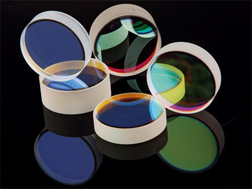
Kingdom of multi-layered mirrors
Today we will get acquainted with multi-layered mirrors, find out why they are needed and how they are modeled using the transfer matrix method.
An ordinary bathroom mirror (and its better-quality counterparts) is nothing more than a thin smooth metal film. When reflected from it, about five percent of the light is lost. Sometimes it is critical - for example, in telecom (the less signal we lose, the less intermediate amplifiers are installed) or in complex optics such as periscopes (if you lose 5% on each mirror, the observer will get very, very little).
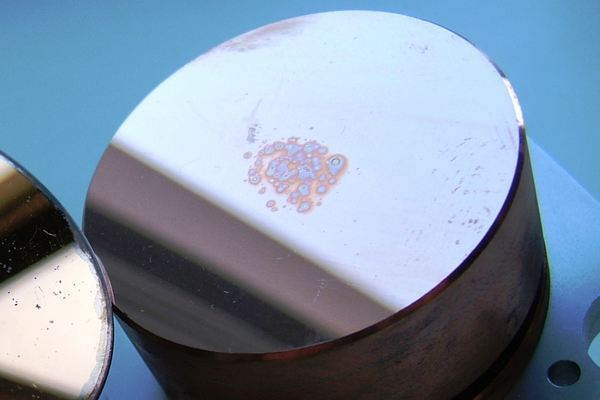
On the other hand, the absorption of light on a mirror causes it to heat up. And if 5% of a laser pointer is something ephemeral, then 5% of an industrial laser for cutting is about a watt, which can noticeably heat a thin film. Still more interesting with pulsed lasers, where peak power is enough to melt a mirror. Like this:
')
Probably many have heard about the enlightenment of optics. This is a tricky lens coating that allows you to reduce the reflection from their front surface to almost zero. That is, the light will not be spent on reflection, but will go completely into the optical system. Physically, this is due to destructive interference from different layers of the antireflection coating.
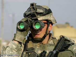
Binoculars with anti-reflective coating.
The same idea can be used in the opposite direction: so that the reflection does not weaken, but on the contrary, increases. We will need a layer cake of two different materials, each quarter-wavelength thick. At each joint of the two materials, part of the light is reflected back. If all the reflections that go outside will have the same phase, constructive interference will occur and the reflected signal will have the highest possible intensity.

Such a “layer cake” is called a dielectric mirror , a multilayer mirror , or a distributed Bragg reflector (in English, distributed Bragg reflector , DBR ). It is “distributed” because the reflection occurs not on one surface, but on several at once. The reflection coefficient can easily reach 99.99%, which means that compared to metal mirrors, losses are reduced by 2-3 orders of magnitude.
Let's take a closer look at the reflection scheme. The incident beam is reflected back on each of the boundaries of the two media. True, each reflected ray also reflects on each of the boundaries, which it passes on the way back — now to the other side. Each of these rays is once again reflected ... hell, how do you count them all?
The transfer matrix method comes to the rescue. Its essence is that we cease to monitor each ray individually, and we only look at the result of their addition. That is, we set the vector describing the wave at each point.
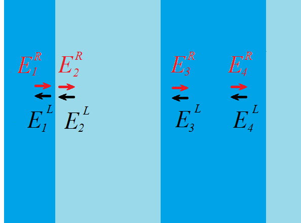
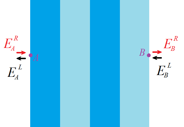
Generally speaking, at each point there are two waves: one propagates to the right (let's call it E R ), the second to the left ( E L ). Then our vector has two elements, and complex ones: we are interested in both the amplitude of the light ( modulus of the number) and its phase (respectively, the phase of the number).

For any two points of the vector will be connected by some linear expression, taking into account the propagation of light through the medium and through the boundaries of two media. You can write this expression using matrices. Basically, we need two matrices. The first (let's call it M 1 ) connects the vectors to the left and right of the interface. The second (M 2 ) describes the wave propagation in a homogeneous medium (between the interfaces).
By combining M 1 and M 2 , we can connect two vectors at any point in space. For example, between points A and B in the figure below the dependence will be as follows:

That is, we simply multiply in a row the matrices for everything that the light passes through (it goes from left to right):
- boundary of air and 1 layer (entrance to the mirror)
- distribution in the first layer
- border 1-2 layers
- distribution in the second layer
- border of 2-3 layers
and so on to exit the mirror. And we get one 2x2 matrix describing the whole mirror at once!
I did not accidentally choose points from two sides of the mirror. At point A, the upper component of the vector (which flies to the right) is the wave that we send to the mirror. The lower component is the reflection that we want to calculate. At point B (immediately behind the mirror), the upper component is the transmission of the mirror, and the lower component is zero because nothing falls from the back side of the mirror. The result is an elementary matrix equation
where r and t are reflection and transmission, respectively. Hence, not forgetting that intensity is the square of amplitude, we get the reflection

In conclusion, we note that for other wavelengths the layers will have a thickness different from a quarter of the wavelength, so the reflection coefficient may change. To find out in which spectral range the mirror will reflect, it is necessary to repeat the calculation for different wavelengths.
The code is straightforward. For each wavelength, you need to calculate M 1 and M 2 , then multiply them as many times as necessary. Since the results for different wavelengths are independent, the calculations are well parallelized on multi-core processors. The code on which the examples were considered below is written in MATLAB. I will mention a few subtleties.
1. M 1 and M 2 for different wavelengths differ due to different refractive indices (this is called the word dispersion ). Typically, the values of the refractive indices are tabulated and vary fairly smoothly, so they are well interpolated by the polynomial.
The problem arises if, starting from a certain wavelength, the material begins to absorb light (say, semiconductors behave this way). Usually for the wavelength at which absorption begins, there is no good tabulated data at all; there is a gap between the values to the left and right of it. In this case, the areas to the left and to the right of the “bad” point are interpolated separately, and the point itself is ignored.
2. If the mirror consists of N pairs of layers, instead of calculating M 1 and M 2 for each layer, you can calculate them once for a pair of layers, and then multiply them N times in the right order. In other words, first calculate the transfer matrix for a pair of layers, and then raise it to the Nth power. Chebyshev polynomials can help with this.
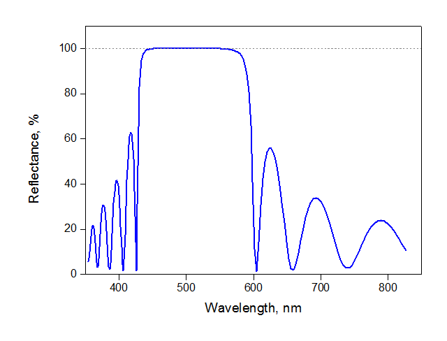
1. Typical reflection spectrum. A simple example is a mirror of alternating layers of TiO 2 and SiO 2 , each 10 times. The reflection reaches a maximum in a certain range: in the picture - from 420 to 600 nm, that is, our mirror works in the blue-green area. Outside the working range, reflection jumps from zero to small values; in these areas the mirror isnot a completely not a mirror, but simply a useless piece of glass. At the maximum, the reflection is approximately 99.97%.
2. More layers - better reflection. By the way, it is considered to be not layers, but their pairs. In the picture below, the red spectrum - 5 pairs of TiO 2 / SiO 2 , blue - 10 pairs. In practice, do not use too much steam, because it increases the production time. Approximate numbers - 5-7 pairs for mirrors in conventional laser diodes and fiber lasers; 20-30 for very specific applications such as quantum optics.

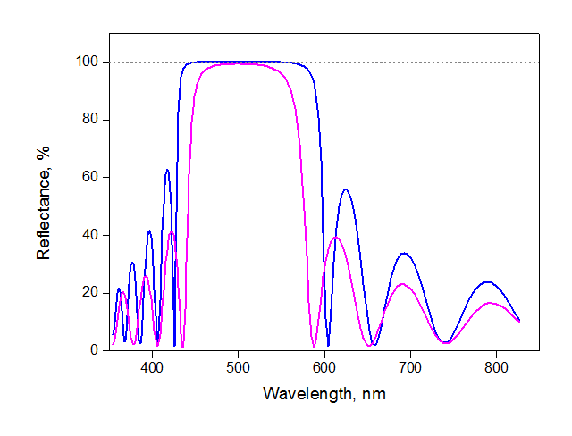
3. The contrast or difference of the refractive indices of the two materials. The larger it is, the less steam is needed for a mirror of the same quality. The picture below shows the spectra of mirrors of 10 pairs of TiO 2 / SiO 2 (blue) and ZrO / SiO 2 (lilac). The latter has a smaller refractive index, therefore the maximum reflection is 99.24% (versus 99.97% for TiO 2 / SiO 2 ) - in other words, the loss in the ZrO / SiO 2 mirror is 25 times larger.
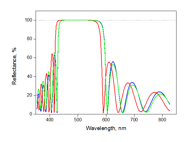
4. Manufacturing accuracy. The layers are extremely thin (0.1-0.2 microns), and small deviations noticeably affect the quality. For the reproducibility of the spectrum, it is critical to monitor not the thickness of each layer, but the thickness of the pair. Let's see what happens to our mirror of 10 pairs of TiO 2 / SiO 2 (blue spectrum) with various errors in manufacturing. If all layers of one material are 10% thicker, and the second one is 10% thinner (green), the thickness of the pair will remain unchanged and the quality of the mirror will change quite weakly. At the same time, the deviation of only one layer by 5% changes the thickness of the pair and noticeably shifts the spectrum (red curve).
Of course, first of all, the transfer matrix method is needed by the corresponding R & D. Laser diodes, fiber lasers, mirrors (ranging from terahertz to soft X-rays), narrow-band filters, and even the clarification of optics are considered to be just that.
Further, we have seen that the interference is very sensitive to the thickness of the layers. In principle, if we approximately know the composition of a certain layered structure, we can determine the thickness of its layers with an accuracy of the order of a nanometer. To do this, measure its reflection spectrum and adjust it by varying the thickness of the layers in the algorithm. It turns out such a system for reverse engineering of layered structures. Moreover, its cost is orders of magnitude less than the cost of an electron microscope with the same resolution.
This results in another application - the feedback on the production of mirrors. The reflection spectrum of the manufactured mirror is easy to measure and compare with the theoretical one. If the differences are significant, the simulation can show exactly what went wrong in the process. Moreover, feedback can be obtained in real time during the manufacturing process: a light bulb shines on the sprayed mirror, and the measured reflection spectrum is displayed on the screen.
The formulas above describe normal reflection (i.e., perpendicular to the mirror). In reality, mirrors that reflect at an angle are often needed. For such calculations, the algorithm is a bit more complicated: you have to add another cycle for different angles.
Slightly more difficult to calculate a concave or convex mirror: it is necessary to separately consider different parts of the surface. Usually in such a situation you have to sacrifice something: a spectrum, angles of reflection, polarization properties. This task is often trusted by a genetic algorithm that is configured to maximize the necessary parameters. For example, you can make a mirror that reflects light from all angles, but the spectrum and quality will not be the best. Or make a mirror with a reflection of about 99.999% - but only for one wavelength and at one angle.
A small plus is that it is not necessary to use a periodic structure: the thickness of the layers can vary as desired (such a mirror is called aperiodic ). You can vary a dozen thickness at once - what a expanse for the genetic algorithm! That is how mirrors for X-ray lithography, which is used in modern technological processes in microelectronics, are calculated.
M. Born, E. Wolf. The Basics of Optics.
On the dxdy forum, a good note about Chebyshev polynomials.
Pictures: KDPV , 1 , 2 , 3 .
What is wrong with ordinary mirrors?
An ordinary bathroom mirror (and its better-quality counterparts) is nothing more than a thin smooth metal film. When reflected from it, about five percent of the light is lost. Sometimes it is critical - for example, in telecom (the less signal we lose, the less intermediate amplifiers are installed) or in complex optics such as periscopes (if you lose 5% on each mirror, the observer will get very, very little).
On the other hand, the absorption of light on a mirror causes it to heat up. And if 5% of a laser pointer is something ephemeral, then 5% of an industrial laser for cutting is about a watt, which can noticeably heat a thin film. Still more interesting with pulsed lasers, where peak power is enough to melt a mirror. Like this:
')
A bit of physics
Probably many have heard about the enlightenment of optics. This is a tricky lens coating that allows you to reduce the reflection from their front surface to almost zero. That is, the light will not be spent on reflection, but will go completely into the optical system. Physically, this is due to destructive interference from different layers of the antireflection coating.
Binoculars with anti-reflective coating.
The same idea can be used in the opposite direction: so that the reflection does not weaken, but on the contrary, increases. We will need a layer cake of two different materials, each quarter-wavelength thick. At each joint of the two materials, part of the light is reflected back. If all the reflections that go outside will have the same phase, constructive interference will occur and the reflected signal will have the highest possible intensity.
Such a “layer cake” is called a dielectric mirror , a multilayer mirror , or a distributed Bragg reflector (in English, distributed Bragg reflector , DBR ). It is “distributed” because the reflection occurs not on one surface, but on several at once. The reflection coefficient can easily reach 99.99%, which means that compared to metal mirrors, losses are reduced by 2-3 orders of magnitude.
A bit of math
Let's take a closer look at the reflection scheme. The incident beam is reflected back on each of the boundaries of the two media. True, each reflected ray also reflects on each of the boundaries, which it passes on the way back — now to the other side. Each of these rays is once again reflected ... hell, how do you count them all?
The transfer matrix method comes to the rescue. Its essence is that we cease to monitor each ray individually, and we only look at the result of their addition. That is, we set the vector describing the wave at each point.
Generally speaking, at each point there are two waves: one propagates to the right (let's call it E R ), the second to the left ( E L ). Then our vector has two elements, and complex ones: we are interested in both the amplitude of the light ( modulus of the number) and its phase (respectively, the phase of the number).
For any two points of the vector will be connected by some linear expression, taking into account the propagation of light through the medium and through the boundaries of two media. You can write this expression using matrices. Basically, we need two matrices. The first (let's call it M 1 ) connects the vectors to the left and right of the interface. The second (M 2 ) describes the wave propagation in a homogeneous medium (between the interfaces).
How it all comes out
Let's start with M 1 . Imagine that light falls on the boundary between two media on both sides. For each of the rays, we can calculate the percentage of reflection and refraction, and then add up the results. Expressions are derived from Fresnel formulas. If the light fell only on the left (E 1 R ), then the reflection and refraction would be given by the formulas
where n 1 and n 2 are the refractive indices of two media. If the light fell only on the right (E 2 L ), we would have accordingly
Combining expressions, we get
Matrix M 2 looks much simpler. Since the rays flying left and right do not interact, the matrix is diagonal. The amplitude of the light does not change - it means that the modulus of the elements of the matrix is equal to 1. Only the phase changes: it increases for the beam to the right, decreases for the left to the left (the minus sign in the exponent). Turns out
where L is the layer thickness, lambda is the wavelength.
By combining M 1 and M 2 , we can connect two vectors at any point in space. For example, between points A and B in the figure below the dependence will be as follows:
That is, we simply multiply in a row the matrices for everything that the light passes through (it goes from left to right):
- boundary of air and 1 layer (entrance to the mirror)
- distribution in the first layer
- border 1-2 layers
- distribution in the second layer
- border of 2-3 layers
and so on to exit the mirror. And we get one 2x2 matrix describing the whole mirror at once!
I did not accidentally choose points from two sides of the mirror. At point A, the upper component of the vector (which flies to the right) is the wave that we send to the mirror. The lower component is the reflection that we want to calculate. At point B (immediately behind the mirror), the upper component is the transmission of the mirror, and the lower component is zero because nothing falls from the back side of the mirror. The result is an elementary matrix equation
where r and t are reflection and transmission, respectively. Hence, not forgetting that intensity is the square of amplitude, we get the reflection
In conclusion, we note that for other wavelengths the layers will have a thickness different from a quarter of the wavelength, so the reflection coefficient may change. To find out in which spectral range the mirror will reflect, it is necessary to repeat the calculation for different wavelengths.
Code and some optimization
The code is straightforward. For each wavelength, you need to calculate M 1 and M 2 , then multiply them as many times as necessary. Since the results for different wavelengths are independent, the calculations are well parallelized on multi-core processors. The code on which the examples were considered below is written in MATLAB. I will mention a few subtleties.
1. M 1 and M 2 for different wavelengths differ due to different refractive indices (this is called the word dispersion ). Typically, the values of the refractive indices are tabulated and vary fairly smoothly, so they are well interpolated by the polynomial.
The problem arises if, starting from a certain wavelength, the material begins to absorb light (say, semiconductors behave this way). Usually for the wavelength at which absorption begins, there is no good tabulated data at all; there is a gap between the values to the left and right of it. In this case, the areas to the left and to the right of the “bad” point are interpolated separately, and the point itself is ignored.
2. If the mirror consists of N pairs of layers, instead of calculating M 1 and M 2 for each layer, you can calculate them once for a pair of layers, and then multiply them N times in the right order. In other words, first calculate the transfer matrix for a pair of layers, and then raise it to the Nth power. Chebyshev polynomials can help with this.
Exponentiation using Chebyshev polynomials.
Let M be a unimodular matrix 2x2 (i.e., its determinant is 1 or -1). Then

Where
 ,
,
a
- Chebyshev polynomials of the second kind.
Where
,a
- Chebyshev polynomials of the second kind.
Interesting results
1. Typical reflection spectrum. A simple example is a mirror of alternating layers of TiO 2 and SiO 2 , each 10 times. The reflection reaches a maximum in a certain range: in the picture - from 420 to 600 nm, that is, our mirror works in the blue-green area. Outside the working range, reflection jumps from zero to small values; in these areas the mirror is
2. More layers - better reflection. By the way, it is considered to be not layers, but their pairs. In the picture below, the red spectrum - 5 pairs of TiO 2 / SiO 2 , blue - 10 pairs. In practice, do not use too much steam, because it increases the production time. Approximate numbers - 5-7 pairs for mirrors in conventional laser diodes and fiber lasers; 20-30 for very specific applications such as quantum optics.
3. The contrast or difference of the refractive indices of the two materials. The larger it is, the less steam is needed for a mirror of the same quality. The picture below shows the spectra of mirrors of 10 pairs of TiO 2 / SiO 2 (blue) and ZrO / SiO 2 (lilac). The latter has a smaller refractive index, therefore the maximum reflection is 99.24% (versus 99.97% for TiO 2 / SiO 2 ) - in other words, the loss in the ZrO / SiO 2 mirror is 25 times larger.
4. Manufacturing accuracy. The layers are extremely thin (0.1-0.2 microns), and small deviations noticeably affect the quality. For the reproducibility of the spectrum, it is critical to monitor not the thickness of each layer, but the thickness of the pair. Let's see what happens to our mirror of 10 pairs of TiO 2 / SiO 2 (blue spectrum) with various errors in manufacturing. If all layers of one material are 10% thicker, and the second one is 10% thinner (green), the thickness of the pair will remain unchanged and the quality of the mirror will change quite weakly. At the same time, the deviation of only one layer by 5% changes the thickness of the pair and noticeably shifts the spectrum (red curve).
Where is it needed
Of course, first of all, the transfer matrix method is needed by the corresponding R & D. Laser diodes, fiber lasers, mirrors (ranging from terahertz to soft X-rays), narrow-band filters, and even the clarification of optics are considered to be just that.
Further, we have seen that the interference is very sensitive to the thickness of the layers. In principle, if we approximately know the composition of a certain layered structure, we can determine the thickness of its layers with an accuracy of the order of a nanometer. To do this, measure its reflection spectrum and adjust it by varying the thickness of the layers in the algorithm. It turns out such a system for reverse engineering of layered structures. Moreover, its cost is orders of magnitude less than the cost of an electron microscope with the same resolution.
This results in another application - the feedback on the production of mirrors. The reflection spectrum of the manufactured mirror is easy to measure and compare with the theoretical one. If the differences are significant, the simulation can show exactly what went wrong in the process. Moreover, feedback can be obtained in real time during the manufacturing process: a light bulb shines on the sprayed mirror, and the measured reflection spectrum is displayed on the screen.
What's next
The formulas above describe normal reflection (i.e., perpendicular to the mirror). In reality, mirrors that reflect at an angle are often needed. For such calculations, the algorithm is a bit more complicated: you have to add another cycle for different angles.
Slightly more difficult to calculate a concave or convex mirror: it is necessary to separately consider different parts of the surface. Usually in such a situation you have to sacrifice something: a spectrum, angles of reflection, polarization properties. This task is often trusted by a genetic algorithm that is configured to maximize the necessary parameters. For example, you can make a mirror that reflects light from all angles, but the spectrum and quality will not be the best. Or make a mirror with a reflection of about 99.999% - but only for one wavelength and at one angle.
A small plus is that it is not necessary to use a periodic structure: the thickness of the layers can vary as desired (such a mirror is called aperiodic ). You can vary a dozen thickness at once - what a expanse for the genetic algorithm! That is how mirrors for X-ray lithography, which is used in modern technological processes in microelectronics, are calculated.
Sources
M. Born, E. Wolf. The Basics of Optics.
On the dxdy forum, a good note about Chebyshev polynomials.
Pictures: KDPV , 1 , 2 , 3 .
Source: https://habr.com/ru/post/259791/
All Articles