OpenEMS dipole antenna simulation

In the previous part it was described how to model the propagation of EME using a simulator
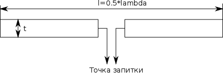
openEMS . Now consider how to calculate something useful. We simulate a dipole half-wave antenna at a frequency of 500 MHz. Modeling in the frequency domain and antenna pattern modeling will be considered. The scheme of this antenna is shown in the figure.


')
A dipole antenna consists of two beams, each of which has a length equal to 1/4 of a wave for a resonant frequency. The antenna is powered from the center. The antenna has a resonance resonance resistance of approximately 75 ohms and a torus-shaped di-gram. More information about the theory of the dipole antenna can be found, for example, in the textbook of Eisenberg or Belotserkovsky. These results we should get after the simulation.

Under the cut, there is a script with a model of a dipole antenna with line-by-line analysis. It is assumed that the reader is familiar with the basics of Matlab / Octave, electrical engineering and antenna theory (he knows what complex resistance, S-parameters and VSWR are).

For those who do not know what is happening here, links to my previous articles:

• openEMS is an open source electromagnetic simulator
• OpenEMS modeling basics

The simulation script must first be saved to a text file with the extension * .m, using your favorite test editor (for example KWrite). Then you need to run Octave from the command line, passing in the name of the script as a parameter. Suppose if our script is called dipole.m, then the simulation starts like this:

octave dipole.m 

If you want to use the graph view from Octave interactively, you must first run Octave from the command line, and then use the source command. It will load the dipole.m script from the current directory.

 source dipole.m 

As a result of the simulation, we want to get:

• The dependence of the input impedance of the antenna at the power point of the frequency.
• Dependence of the antenna CWS at the power point on the frequency for a 50 Ohm source
• DN in polar coordinates
• 3D NAM in spherical coordinates

Let's start the line by line parsing script. The openEMS documentation suffers from spaces, so something had to be thought out for itself.

So at the beginning of the script we clear all variables:

 close all; clear; clc; 

Now you need to announce the name of the XML file that contains the task for the simulation and the temporary directory in which the simulation results will be stored. Files with the results of calculations reach 100 MB, so you need to take care of disk space.

 physical_constants SimPath = 'tmp'; SimCSX = 'tmp.xml'; 

Now we begin the description of the parametric model of the antenna. This means that when changing parameters (for example, the calculated resonant frequency), Matlab / Octave will automatically recalculate all antenna sizes. The grid spacing is set equal to 1/50 wavelength.

 f_max = 0.5e9; #    lambda = c0/f_max; #   step=lambda/50; #   

As you remember from physics, wavelength and frequency are related through the speed of light.
c0

We declare simulation space (SimBox) - a cube with an edge equal to
doubled wavelength (2 * lambda). Fill the space with a grid
mesh

 CSX = InitCSX(); mesh.x = -lambda:step:lambda; mesh.y = -lambda:step:lambda; mesh.z = -lambda:step:lambda; SimBox = [2*lambda 2*lambda 2*lambda]; CSX = DefineRectGrid(CSX,1,mesh); 

Now we set the excitation source. In the last part, we used a sinusoidal source of a fixed frequency. openEMS first performs the calculation in the time domain, and then recalculates the result in the frequency domain. Therefore, in order to simulate the frequency properties of the system, you need a source with an extended spectrum. The Gaussian impulse is available as such a source in openEMS.

So, first, we assign the variables in which we will store the parameters of the Gaussian pulse. You must specify the center frequency of the Gaussian pulse spectrum and half the width of the spectrum. We will model our antenna in the frequency range from 200 MHz to 600 MHz. Therefore, the center frequency will be 400 MHz, and the width of the spectrum + -200 MHz from the center frequency.

 f0 = 400e6; fc = 0.5*f0; FDTD = InitFDTD('NrTS',30000); FDTD = SetGaussExcite(FDTD,f0,fc); 

The FDTD space is initialized using the InitFDTD () function. The second parameter is to pass the number of samples in the time domain to it. It must be chosen in such a way that it exceeds the pulse duration in sampling steps. Usually 30,000 is enough. Otherwise, we will receive an error message, which states that the calculation interval is less than the duration of the Gaussian pulse.

Now you need to set the boundary conditions. We are modeling an antenna in free space, so it will be surrounded on all sides by an absolutely absorbing MUR dielectric:

 BC = {'MUR','MUR','MUR','MUR','MUR','MUR'}; FDTD = SetBoundaryCond(FDTD,BC); 

Now we declare the geometry. The process of describing geometry for those familiar with, for example, HFSS looks unusual and unusual.

The dipole will consist of two conducting parallelepipeds between which the excitation source is connected. The thickness of the dipole rays may be less than the grid pitch. As the theory says, the greater the thickness of the dipole antenna, the wider its bandwidth. All our geometry is parameterized and will be automatically recalculated when changing parameters. This is the advantage of the Matlab / Octave simulator.

 t = step/4; #    (1/200  ) CSX = AddMetal(CSX,'right_beam'); #    start = [t -t -t]; #   stop = [lambda/4 tt]; #   CSX = AddBox(CSX,'right_beam',1,start,stop); #     

The coordinates of points in space are specified in openEMS as a matrix-row of three components, which follow the order [xyz].

The AddMetal () function adds some metal object. The created object must be associated with some geometric object. The AddBox () function adds a box. The penultimate and last parameters are the coordinates of its extreme vertices. The third parameter is the priority. His appointment remains unclear to me. You can always set it to 1. The second parameter is the name of the parallelepiped material object. We have to use the 'right_beam' object that we created earlier.

Similar action for the left beam:

 CSX = AddMetal(CSX,'left_beam'); start = [0 -t -t]; stop = [-lambda/4 tt]; CSX = AddBox(CSX,'left_beam',1,start,stop); 

Now you need to power the antenna. To power the antenna is a special object called the port (Lumped Port).

There is also a distributed port, which is an area of ​​space from which EMW is distributed. The distributed port was used in the second part.

We need to use a regular port. It corresponds to the case of powering the antenna from the voltage source. The voltage source is the previously announced Gaussian pulse. The port consists of two points in space, between which the terminals of the virtual voltage source are connected. First, we declare these two points. They should lie on the surface of the dipole rays:

 start = [0 0 0 ]; #    stop = [step 0 0]; 

Now we will declare the output impedance of the source:

 R = 50; 

And you can add the actual port:

 [CSX port] = AddLumpedPort(CSX,1,1,R,start,stop,[1 0 0],true); 

The AddLumpedPort () function has 8 parameters. Consider them in more detail:

• The second parameter is priority. You can put in 1
• The third parameter is the serial number of the port. Maybe a few
  ports.
• The fourth parameter is the output impedance of the source
• The fifth and sixth parameters - port connection points
• The seventh parameter is the direction of the signal. Vector of three components
  which shows the direction of the signal in [xyz] format. We have
  the signal is directed along the x axis.

Now you need to specify the area in which the field emitted by the antenna will be calculated. openEMS calculates the field in the near zone, and then using the post-processor NF2FF recalculates it in the field in the far zone. The antenna DN is calculated from the field in the far zone. The area in which the field is calculated is to be taken equal to the modeling area, having necessarily stepped inside several grid steps from the border.

 SimBox = SimBox-step*4.0; #    [CSX nf2ff] = CreateNF2FFBox(CSX,'nf2ff',-SimBox/2,SimBox/2); 

Everything! Geometry set. You can write a job file for openEMS and see the result in the AppCSXCAD interactive viewer.

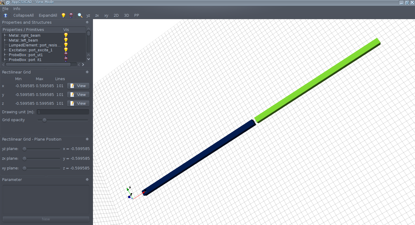
 mkdir('tmp'); SimPath = 'tmp/tmp.xml' WriteOpenEMS(SimPath,FDTD,CSX); CSXGeomPlot(SimPath); 

If everything is done correctly, we will see the following picture (the port is visible in the dipole gap):



Now we run openEMS.

 RunOpenEMS('tmp','tmp.xml'); 

The calculation takes quite a long time. After calculation are created for the structure:

• port - contains information about the characteristics of the antenna in
  frequency domain
• nf2ff - contains information about the antenna NAM

We need to extract from the structure of the port information about the input impedance of the antenna and the reflection coefficient S11. To do this, you need the following structure fields
port:

• port.uf.tot - Full voltage at the port terminals
• port.if.tot - Total current flowing through the port
• port.uf.inc - Amplitude of incident wave voltage
• port.uf.ref - amplitude of the voltage of the reflected wave

Tepr using formulas known from the course of radio engineering, we calculate the input resistance Zin and the reflection coefficient at the input S11 (it can be recalculated into
standing wave ratio - SWR). Now you can plot the graphics Zvh (active and reactive parts), VSWR and S11, using standard tools Matlab / Octave This piece of code does not require explanation.

 freq = linspace(f0-fc,f0+fc,501); #   port = calcPort(port,'tmp',freq); #   Zin = port.uf.tot ./ port.if.tot; S11 = port.uf.ref ./ port.uf.inc; subplot(3,1,1); plot(freq/1e6,real(Zin),freq/1e6,imag(Zin)); #   R  X legend('Re(Zin)','Im(Zin)'); subplot(3,1,2); plot(freq/1e6,S11); #   S11 swr = (1+abs(S11))./(1-abs(S11)); #     [swr_min idx] = min(swr); [Xmin idx1] = min(abs(imag(Zin))); #    fr = freq(idx); fr1 = freq(idx1); Zr = Zin(idx); Zr1 = Zin(idx1); disp("Minimum SWR frequency:"); #    disp(fr); disp("Resonant frequency (jX=0)"); disp(fr1); disp("Impedance at minimum SWR"); disp(Zr); disp("Impedance at resonant frequency"); disp(Zr1); disp("Minimum SWR:"); disp(swr_min); subplot(3,1,3); semilogy(freq/1e6,swr); 

We get the following antenna parameters. It is seen that the resonance frequency went down from the calculated one. Antenna resistance at a resonance of 71.2 ohms is almost like in textbooks, the deviation is caused by the dipole thickness.

 Minimum SWR frequency: 427200000 Resonant frequency (jX=0) 431200000 Impedance at minimum SWR 68.7692 - 6.5511i Impedance at resonant frequency 71.18555 - 0.45064i Minimum SWR: 1.4013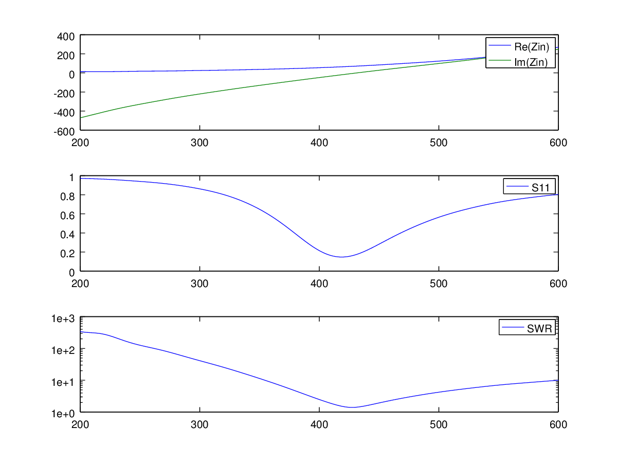 

Now we calculate the DN in polar coordinates. The last two parameters of the function CalcNF2FF () are the range of angles within which the pattern is viewed. By the third parameter, it needs to transmit the frequency at which the pitch pattern is calculated.
We get the following graphics:

 nf2ff = CalcNF2FF(nf2ff,'tmp',fr,[-180:2:180]*pi/180,[0 90]*pi/180); figure polarFF(nf2ff,'xaxis','theta','param',[1 2],'normalize',1); 

DN in Cartesian coordinates:

 figure plotFFdB(nf2ff,'xaxis','theta','param',[1 2]);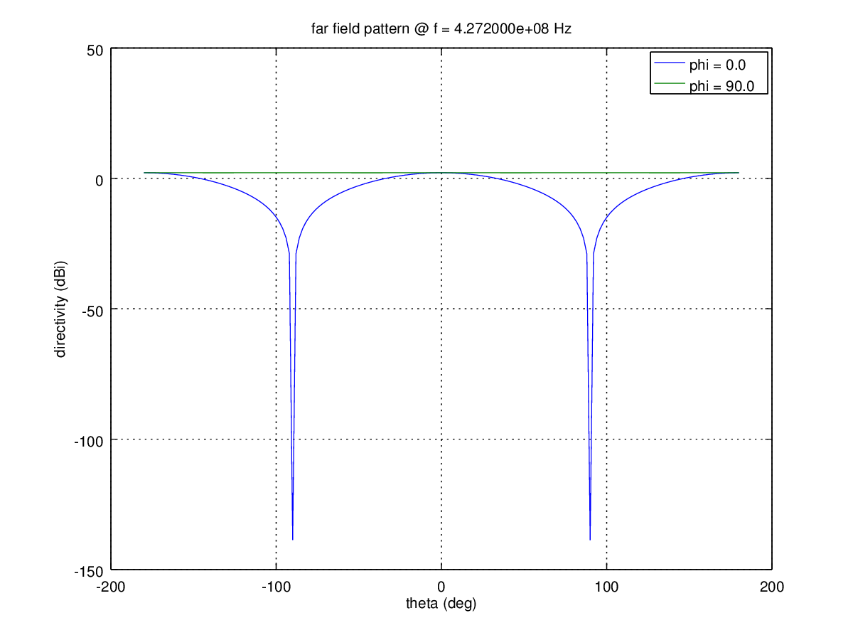 

 thetaRange = (0:2:180); phiRange=(0:2:360)-180; nf2ff = CalcNF2FF(nf2ff,'tmp',fr,thetaRange*pi/180,phiRange*pi/180,'Verbose',1,'Outfile' ,'3D_Pattern.h5'); figure plotFF3D(nf2ff,'logscale',-20);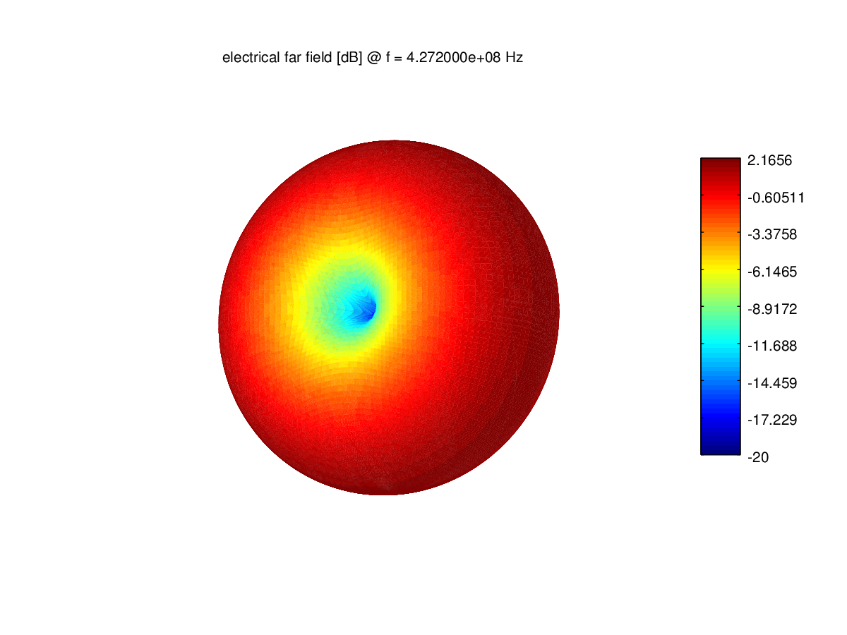 

Spatial DN has the shape of a torus as in the textbooks on antennas. Coefficient
2.1 dB antenna gain.

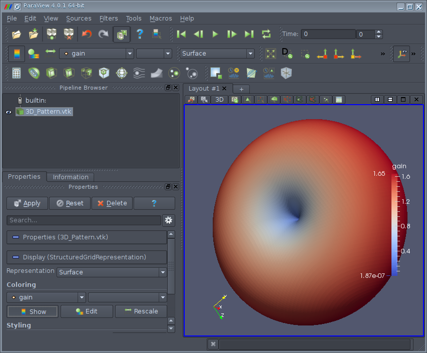
You can also create a * .vtk file so that you can view it later with Paraview:

 E_far_normalized = nf2ff.E_norm{1} / max(nf2ff.E_norm{1}(:)) * nf2ff.Dmax; DumpFF2VTK(['tmp/3D_Pattern.vtk'],E_far_normalized,thetaRange,phiRange,'scale', 1e-3); 

This is how the DN looks in Paraview (you need to open the 3D_Pattern.vtk file):



We simulated a dipole antenna in the frequency range from 200 to 600 MHz. As you can see, the simulation gives results close to the theory and allows to take into account the influence of the deviation of the parameters of the dipole from the ideal. Those who have at hand HFSS can check the result.

In conclusion, we give our entire script:



Perhaps the continuation should ...