Sensors and microcontrollers. Part 1. The materiel
 In the era of ready-made debug boards and thousands of ready-made modules for them, where it is enough to take a couple of blocks, connect them together, and get the desired result, not everyone understands the basics of circuitry, why and how it works, and most importantly - what to do if it works not this way.
The circuitry hub has just opened, so, as Beauford Mad Dog Tannen said
The court building is already being built, so it's time to hang someone.
In this cycle I will talk about sensors - as an important element of the control system of a certain object or those. process.
I will lead all my narration on the practical issues of implementing digital control systems based on microcontrollers.
The manual does not claim to be a universal question.
Although after my abstract climbed over 20 pages of text, I decided to split the article into the following parts:
- Part 1. Mat. part. In it, we will consider a sensor that is not tied to any particular measured parameter. Consider the transfer function and the dynamic characteristics of the sensor, let's deal with its possible connections.
- Part 2. Climate control sensors . In it, I will consider the features of working with sensors of temperature, humidity, pressure and gas composition
- Part 3. Sensors of electrical quantities. In it, I touch the measurement of current and voltage
Introduction
In the control system of a technological installation, the reading of the current readings of a certain value — temperature, humidity, pressure, liquid level, voltage, current, etc. It is carried out with the help of sensors - devices and mechanisms designed to convert the external influence signal into a form that is understandable to the control system. For example, a humidity sensor generates an electrical signal proportional to the current value of air humidity.
')
As a rule, sensors are not used by themselves, but are part of the control system, providing a feedback signal.
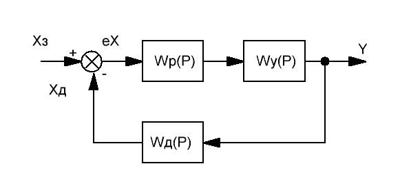
Figure 1. Typical scheme of a closed control system
Figure 1 shows a typical scheme of the regulatory system. There is a reference signal Xz , which is compared with the output signal obtained by means of a sensor having a transfer function Wd (p) . The control error is fed to the regulator, which, in turn, generates a control signal of the actuating unit, which forms the output signal Y. [1]
A simple example is a centrifugal engine speed regulator, where the sensor is a platform with balls, which, rotating, sets one or another position of the fuel rail. The valve, controlled by this rail, regulates the amount of fuel supplied to the engine. The target signal will be the required speed value.
1.1 Sensor classification
Sensor classification is very diverse. I will give only a part of it based on [4].
All sensors are divided into two main classes:
- Passive, which do not need an external source of electricity, and in response to the input action generate an electrical signal. Examples of such sensors are thermocouples, photodiodes, and piezoelectric sensing elements.
- Active, which require for their work an external signal, called the excitation signal. Since such sensors change their characteristics in response to changes in external signals, they are called parametric. Examples of active sensors are thermistors, the resistance of which can be calculated by passing an electric current through them.
It should be noted that the alternative classification is also found in the literature, when the generator sensors are defined as Active, and Parametric Sensors - as Passive. Hereinafter I am guided by the option according to the Fariden reference book.
Another important criterion for us is the choice of data reference point. Thus, sensors are
- Absolute, the measured value of a physical quantity which does not depend on the measurement conditions and the external environment.
- Relative, when the output signal of such a sensor in each case is interpreted differently.
A striking example is again a thermistor, whose resistance directly depends only on the temperature of the object being measured, and a thermocouple, the output voltage of which depends on the temperature difference between the hot and cold ends.
In the development of electronic equipment, an important factor in the characteristics of the sensor is also the nature of the output signal.
- The analog sensors at the output have a continuous output signal, for which removal it is necessary to use an analog-to-digital converter, after which it is necessary to convert the ADC value into the format of the measured value.
- Digital sensors, information from which is removed using various digital interfaces. As a rule, information is available directly in the format of the measured value and does not require additional transformations.
- Discrete sensors that have only two options for the signal at the output of the sensor channel - log 0. and log. 1. An example of such a sensor is a limit switch having closed and open states. A discrete sensor can have several output channels, each of which is in one of two states. For example, a 12-bit absolute position sensor.
- Pulse sensors that generate output signal pulses, the amplitude or duration of which depends on the measured value. For example, an incremental position sensor generates a Gray code at the output. At the same time, the higher the shaft rotation speed of the sensor, the higher the signal frequency will be at the output, which will allow determining the shaft rotation speed with high accuracy.
2 Sensor Characteristics
Most sensors have a complex procedure for converting the measured value into an electrical signal. For example, in a strain gauge pressure sensor, the measured value acts on the sensitive element, changing its resistance. After applying the excitation signal, the voltage drop across the resistor will allow you to indirectly determine its resistance and, based on the dependence of the resistance on pressure, calculate the measured value.
For a developer, a sensor is a black box with known signal ratios between inputs and outputs.
2.1 Range of measured and output values
The range of measured values indicates what the maximum value of the input signal can be converted by the sensor into an output electrical signal, without going beyond the limits of the established errors. These figures are always given in the specification for the sensor, at the same time displaying the possible accuracy of measurements in one or another range.
It should be understood that some sensors, when the input signal exceeds the maximum values, will simply become saturated and will return incorrect data. Other sensors (for example, temperature sensors) can fail. In the future, for each type of sensor will be given their recommendations.
The range of output values of the sensor is the minimum and maximum voltage that the sensor is able to produce at the minimum and maximum external exposure. Since we consider sensors that convert an input signal into an electrical one, the range of output values of the sensor will be determined by the voltage it produces, or the current passing through it. One of our tasks when connecting a sensor will be to match the output range of the sensor with the input range of the measuring path.
2.2 Transfer function - static and dynamic characteristics
When working with the sensor is required to know the ratio of the levels of the signals at the input and output. The ratio Wd (p) = Y (p) / X (p) in an operator form is the transfer function of the sensor and uniquely determines the characteristics of the sensor in statics and dynamics.
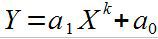
The equation Y (p) = Wd (p) * X (p) in the real plane, i.e. the function Y = f (x) will be a static characteristic
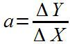
The static characteristic can be linear and will be defined as:
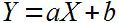 (one)
(one)Where a is the slope of the straight line determined by the sensitivity of the sensor and b is the constant component (that is, the output signal level when there is no signal at the input)

Figure 2. Linear dependence
In addition to sensors with linear dependence, there may be sensors with a logarithmic dependence, with an equation of the form
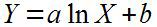 (2)
(2)Exponential:
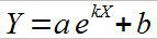 (3)
(3)Or power:
 (four)
Where k is a constant number.
There are sensors with more complex characteristics. But there is documentation.
However, the transfer function also reveals what properties the sensor has in dynamics, i.e., how quickly and precisely the sensor performs the output signal when the input value changes rapidly. Practically every real sensor has an energy storage device in itself - a capacitor, a mass, etc. Consider the sensor behavior, the dynamic characteristics of which are described by a first order equation:
 (five)
In the theory of automatic control, there are two test input signals. This is a single function — the feed at zero time is one, and the delta function is a feed of a signal of infinite amplitude and infinitely small duration.

Figure 3. Single and delta functions
Inertia-free, I mean the ideal sensor will exactly repeat the input signal form. The real sensor described by the formula (5) will give the following reaction:

Figure 4. Reaction of the first-order aperiodic link to test signals
It should be noted that the value at the output of the sensor will correspond to that supplied at the input only after the completion of the transition process, which will last 3-4 τ , where τ is the time constant of our link. When t = 1τ , the output value will reach

It is easy to calculate that at t = 2τ the output value will be 86%, and at t = 3τ - 95% and the transition process will be considered complete.
Thus, it should be understood that, for example, the same temperature sensor will react to a change in the ambient temperature with some delay due to the fact that there is a housing between the sensor and the environment, which must absorb heat and heat. It takes time.
Of course, inertial sensors can be described by more complex equations, for example, they can be second-order aperiodic units, have a reaction delay, etc. The behavior of such units is described in detail in [1].
2.3 Accuracy, nonlinearity
One of the important characteristics of the sensor is its accuracy in the range of measured values. The output signal of the sensor corresponds to the value of the measured value with some certainty, called the error.
For example, a temperature sensor has an accuracy of ± 2 degrees. This means that at a real temperature of the object being measured at 100 degrees, the permissible readings of this temperature sensor are in the range of 98 to 102 degrees.
Sensor error is different.
There are additive and multiplicative error.
The additive error is constant over the entire measurement range.
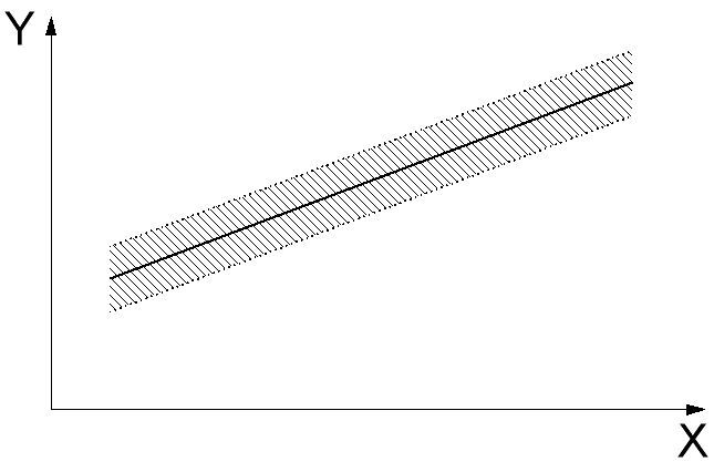
Figure 5. Additive error
Multiplicative linearly depends on the level of the measured value:
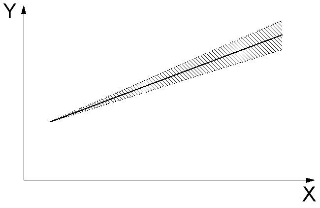
Figure 6. Multiplicative error
In addition, there is a non-linearity of the sensor in the measured range. Depending on the current measurement range, the slope of the transfer function varies within certain limits. In this case, the specification indicates either the curves of variation of accuracy over the range, or the worst indicators of nonlinearity in one or another range.
Figure 7. Sensor nonlinearity
In addition, some sensors have a hysteresis effect, when for the same input signal, after increasing and decreasing, the output signal values are different. A typical cause of hysteresis is friction and structural changes in materials. Sensors based on ferromagnetic materials are subject to the greatest hysteresis effect.
To improve the accuracy and compensation of additive and multiplicative error, the sensor calibration process can be performed. For example, for a linear sensor, it is necessary to determine the readings at two points at different ends of the operating range with a known accuracy. For some sensors, calibration data may be provided in the passport for each specific instance. For the calibration procedure, you can use more accurate equipment, you can use the standard (for example, black body, reference kilogram, etc.). Accuracy after calibration naturally will not exceed the accuracy of the standard.
2.4 Sensor sensitivity, resolution and dead zone
The sensor dead zone is the sensor insensitivity in a certain range of input signals. Within this zone, the output readings are incorrect.
For example, in Figure 2, the output value for all values from 0 to x0 is not defined. For example, some current sensors that have zero voltage at the output at currents lower than, for example, 10 mA, sin with this feature.
In the rest of the range, there is a certain sensitivity of the sensor, i.e., how strong is the increase in the output signal for a change in the input signal. that is, sensitivity is defined by the following formula:
For a linear sensor, the sensitivity will be constant over the entire measured range.
The resolution shows how small a change in the measured value can cause a change in the output signal. For example, some incremental position sensor has a resolution of 1 degree. Analog sensors have an infinitely large resolution, since in their output signal it is impossible to determine the individual steps of its change.
3 Sensor connection method
Depending on the type of sensor, it is connected to the measuring path in different ways.
Connection of the passive sensor
Since the passive sensor without any help in response to an external effect independently produces an electrical signal for us, we need to consider this signal.
Depending on whether our sensor is a current source or voltage source, the connection method will differ.
For example, a thermocouple is a voltage source - the voltage at the output does not depend on the magnitude of the output current (within reasonable limits of course). Our task is to measure the EMF produced. Since the measuring path will have some final resistance, the wiring diagram will be as follows:
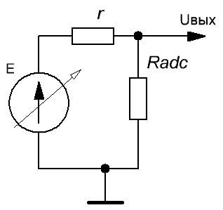
Figure 8. Connecting the voltage source to the ADC
If Radc is much greater than the internal resistance r , then the voltage drop across it will tend to zero and the voltage at the ADC input will tend to the value of the EMF.
In the second part, I will consider in detail the thermocouple, as one of the most accurate and fast sensors.
Another case is if our sensor is a current source, that is, the voltage it generates depends on the current passed through the load.
Connecting the sensor is similar:
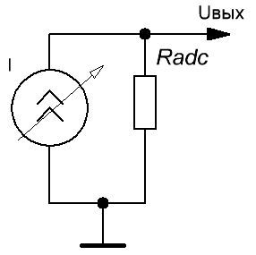
Figure 9. Connecting the current source to the ADC
However, the load resistance of the current source should now tend to zero. For this, the sensor is shunted by a resistor of the necessary resistance, thereby turning the current source into a voltage source:
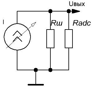
Figure 10. Proper connection of the current source to the ADC
The resistance of resistor R is calculated as the quotient by dividing the maximum voltage applied to the ADC input by the maximum current that the sensor is able to output
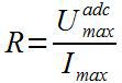
The most vivid image of such a sensor is a current sensor.
ATTENTION: sensors that have a replacement circuit in the form of a current source should always be shunted by resistance and not be allowed to break the shunting circuit in the presence of an arbitrarily small input. Otherwise, the same current sensor generates voltages in kilovolts at the free terminals of the secondary winding before the breakdown of the measurement circuit or the sensor itself. Modern current sensors are tested at a voltage of 1kV or more, so getting 2-3 kV at the output, and getting into them with your finger is not the most difficult task.
Active sensor connection
Consider active sensors, which are variable resistance. In particular, these are thermistors, strain gauges and other similar sensors. To measure the resistance of the sensor, it must be connected to a current source and determine the voltage drop across it:
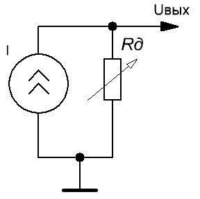
Figure 11. Connecting the sensor to an unregulated current source
The current source produces a constant current of a known value. Then, the output voltage will be determined by the formula:
 (7)
(7)For example, we calculate the output voltage value at a current source of 10 mA if our sensor changes the resistance from 0.1 kΩ to 1 kΩ. Then the maximum output voltage will be equal to
 (eight)
That quite corresponds to the required value of voltage for an analog control system based on operational amplifiers.
Where to get the current source? It so happens that it is built into the microcontroller itself. For example, in the ADuCM360 / 361 microcontrollers there are two embedded current sources of 0.01-1 mA. It is true there they have a diagnostic task - applying a small current through the sensor circuit can be convinced of its presence and serviceability.
Of course, we are used to using a voltage source with a divider:

Figure 12. Connecting the sensor to a voltage source with a divider
Speaking of purity, the U-R1 chain forms the same current source, only its parameters depend on the load - Rd . The output voltage will be determined by the following formula:
 (9)
(9)And here the main problem of this method comes up - you can’t get rid of the resistance of our sensor in the denominator and the readings become non-linear, unlike, by the way, the first option.
The question is - what should be the resistance of R1 ? It should provide the maximum output voltage range. i.e. with known values of the minimum and maximum resistance of the sensor Rd1 and Rd2 , abs (Uout1 - Uout2) -> max
On the other hand, the maximum output voltage we have is limited to the input circuits of the measuring device. For example, the input of a microcontroller with 5V power supply must be energized, for example, no more than 2.5V. I note that if the maximum possible voltage applied to the ADC input is less than the supply voltage, then we will be able to feed it there.
If our sensor changes the resistance from 0.1 kΩ to 1 kΩ, then we take the resistance of resistor R1 equal to the upper limit of the sensor resistance. Then Uout can vary from 1 / 11Uin to 1 / 2Uin. In absolute figures of this example - from 0.45 to 2.5V. And we use such values (2.5-0.45) / 2.5 = 82% of the entire ADC range, which is pretty good.
Another sensor can be plugged into the measuring bridge and measure the voltage difference in its shoulders:
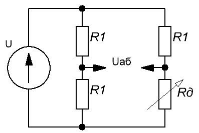
Figure 13. Sensor in the measuring bridge
In this case, we work with a differential ADC, measuring the potential difference Uab . It will be equal to:
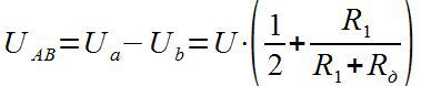 (ten)
(ten)Moreover, the resistance of the resistor R1 may be such that Uab could be negative. There are sensors, the internal scheme of which is already a balanced bridge with the necessary characteristics. Later I will look at examples of such sensors.
There are more convenient to use sensors. They give the necessary analog signal and without dancing with resistors. For example, the analog humidity sensor HIH-4010-004 is a three-output case, 5V power supply, line output. This miracle connects like this:
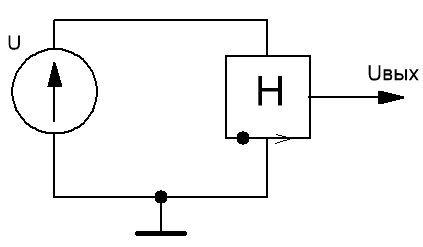
Figure 14. Connection of the HIH-4010-004 humidity sensor
Two wires to the reference voltage source, output - to the ADC of the microcontroller.
Connection of digital sensors according to the standard 1-Wire
1-Wire is a bidirectional low-speed digital data bus that requires only two wires - data wire and ground. The bus is quite simple to use, it supports parasitic powering of devices from the line and allows you to connect in parallel many devices of the same type, like temperature sensors (all your favorite DS18B20), or identification chips (iButton).
Parasitic nutrition is organized as follows:
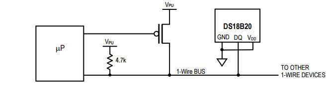
Figure 15. Parasitic powering of 1-Wire bus devices
And this is the usual active power supply of the device, when it’s close to the source.

Figure 16. Powering a 1-Wire device from an external source
The number of sensors connected in parallel is actually limited only by the line parameters.
Perhaps hot plug and identification on the go. Moreover, the computational complexity of the identification algorithm O (log n)
In more detail with this protocol we will work in the second part.
In the meantime, about the protocol itself can be read on the classic link: http://datasheets.maximintegrated.com/en/ds/DS18B20.pdf
Connection of digital sensors according to I2C (Twi) / SMBus standard
If 1-Wire required one data wire, then this bus, according to the name Two-Wire Bus - two.
One of the wires - SCL will be clocking, on the second - SDA, half duplex data will be transmitted.
An open collector tire, therefore both lines need to be pulled to power. The sensor will connect as follows:

Figure 17. Sensor connection via I2C
The total number of devices that can be connected to the I2C bus is 112 devices with 7-bit addressing. Each device is actually allocated two consecutive addresses, the least significant bit is set to read or write. There is a strict tire capacity requirement - no more than 400pF.
Commonly used speeds are 100 kbps and 10 kbps, although the latest standards allow speeds of 400 kbps and 3.4 mbps.
The bus can work as with an irremovable master, there and with the transfer of the flag.
A huge amount of information on the protocol can be found at this link: http://www.esacademy.com/en/library/technical-articles-and-documents/miscellaneous/i2c-bus.html
SPI Digital Sensor Connection
Requires at least three wires, works in full duplex mode - i.e. organizes simultaneous data transfer in both directions.
Communication lines:
- CLK is the clock line.
- MOSI - master output, slave input
- MISO - master input, slave exit
- CS - chip selection (optional).
One of the devices is chosen by the master. It will be responsible for clocking the bus. Connection is made in a cross way:
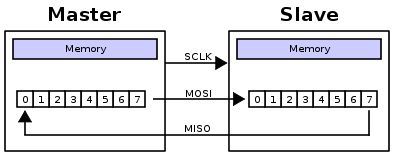
Figure 18. SPI connection and the essence of the transfer
Each device in the chain contains its own shift register data.With the help of clocking signals, after 8 clocks, the contents of the registers change places, thereby carrying out data exchange.
SPI - The fastest data transmission interface presented. Depending on the maximum possible clocking frequency, the data transfer rate can be 20, 40, 75 Mb / s and higher.
The SPI bus allows you to connect devices in parallel, but here a problem arises - each device requires its own CS line to the processor. This limits the total number of devices on a single interface.
The main difficulty in configuring SPI is to set the clocking signal polarity. Seriously. SPI , .
SPI SPI AVR MSP430 http://www.gaw.ru/html.cgi/txt/interface/spi/index.htm
4
- .
. , , , , , .
, — . :

19.
:
1. , , .
, — , . — .
:
Sensor.Start();// delay(MINIMAL_SENSOR_DELAY_TIME);// int var = Sensor.Read();// Option 2 . they started the measurement mode, returned to other tasks, after a while the interruption worked, the data was counted.
One of the best options. But the most difficult:
void Setup(){ TimerIsr.Setup(MINIMAL_SENSOR_DELAY_TIME);// int mode = START;// Sensor.Start();// } TimerIsr.Vector(){// if (mode == START{ mode = READ; var = Sensor.Read();// , } else { mode = START; Sensor.Start();/// , } } Looks good. allows you to vary the time between measurement cycles and read cycles. for example, the gas composition sensor should have time to cool down after previous measurements, or to have time to heat up during measurements. These are different periods of time.
Option 3: Read the data, launched a new round.
If the sensor allows you to start a new measurement cycle after reading the data, then why not - we will do the opposite.
void Setup(){ TimerIsr.Setup(MINIMAL_SENSOR_DELAY_TIME);// Sensor.Start();// } TimerIsr.Vector(){// var = Sensor.Read();// Sensor.Start();/// A great way to save time. and you know what - this method works fine without interruption. Digital sensors store the calculated value until the power is turned off. And given the fact that it is often not necessary to read signals from the humidity sensor due to its inertia of 15 seconds, you can do this:
void Setup(){ Sensor.Start();// while(1){ // var = Sensor.Read();// Sensor.Start();/// } } It may also be such an option that our sensor independently launches a new measurement cycle and then, using an external interrupt, it reports the completion of measurements. For example, the ADC can be configured to automatically read data at a frequency of N Hz. On the one hand, in the interrupt handler, it will be sufficient to implement only the process of reading new data. On the other hand, it is possible to use the ADC interrupt with the Direct Memory Access mode (DMA). In this case, at the interrupt signal, the peripheral ADC module at the hardware level will independently copy data into a specific memory cell into RAM, thereby ensuring maximum data processing speed and minimal impact on the work program (no need to go into the interrupt, call the handler, etc.).
But using DMA is far beyond the scope of this cycle.
Unfortunately, the first method is universally used in libraries and examples for Arduino, it does not allow this platform to properly use the resources of the microcontroller. But it is easier to write and debug.
4.1 Working with ADC
Dealing with analog sensors, we deal with ADC. In this case, the ADC is built into the microcontroller. Since the ADC is essentially the same sensor - converts an electrical signal into an information signal - for it, everything described above in section 2 is valid. The main characteristics of the ADC for us are its effective capacity, sensitivity, reference voltage and speed. At the same time, the output value of the ADC conversion will be a number in the output register, which must be converted to an absolute value in units of the measured value. In the future, for individual sensors, examples of such calculations will be considered.
4.1.1 Reference Voltage
The reference voltage of the ADC is the voltage to which the maximum output value of the ADC will correspond. The reference voltage is supplied from a voltage source, both embedded in the microcontroller and external. The accuracy of the ADC readings depends on the accuracy of this source. The typical reference voltage of the integrated source is equal to the supply voltage or half the supply voltage of the microcontroller. There may be other values.
For example, the table of possible values of the reference voltage for the Atmega1280 microcontroller:
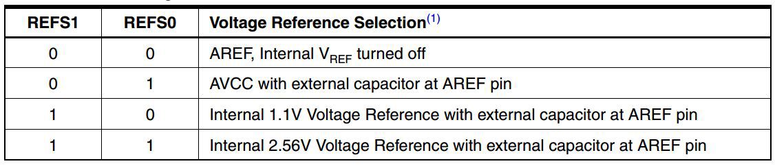
Figure 20. The selection of the reference voltage for the ADC microcontroller Atmega1280
4.1.2 ADC resolution and sensitivity
The ADC resolution determines the maximum and minimum values in the output register with the minimum and maximum input effects of an electrical signal.
It should be noted that the maximum digit capacity of the ADC may not correspond to its effective digit capacity.
Some of the lower digits may be given to noise. Let us turn to the ADuCM360 microcontroller datasheet, which has a 24-bit ADC with an effective bit depth of 14 bits:
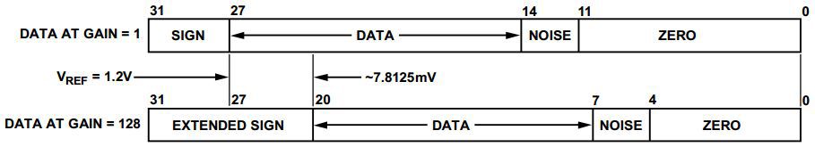
Figure 21. Assignment of the bits of the ADC data register
As can be seen from the figure, in a 32-bit register, a part is allocated to a sign, a part to zeros and a part to noise. And only 14 bits contain data that have the specified accuracy. In any case, these data are always indicated in the documentation.
The sensitivity of an ADC determines its sensitivity. The more intermediate the output voltage steps, the higher the sensitivity will be.
Suppose the reference voltage is ADC Uop . Then, the N-bit ADC, having 2N possible values, has a sensitivity
 (eleven)
Thus, for a 12-bit ADC and a reference voltage of 3.3V, its sensitivity will be 3.3 / 4096 = 0.8 mV
Since our sensor also has a certain sensitivity and accuracy, it would be nice if the ADC has the best performance.
4.1.3 ADC speed
The speed of the ADC determines how quickly the readings are read. A sequential approximation ADC requires a certain number of clock cycles to digitize the input voltage level. The greater the bit depth, the longer it takes, respectively, if by the end of the measurement the signal level has time to change, it will affect the accuracy of the measurement.
The speed of the ADC is measured in the number of data samples per second. It is defined as the frequency of the ADC clock signal divided by the number required for the measurement. For example, having a clocking frequency of 1 MHz ADC and 13 clocks to take readings, the ADC speed will be 77 kilo-samples per second. For each variant of the bit it is possible to calculate its speed. The technical documentation usually indicates the maximum possible clock frequency of the ADC and its maximum speed at a certain bit depth.
4.2 Digital sensors
The main advantage of digital sensors over analog - they provide information about the measured greatness in finished form. The digital humidity sensor will return the absolute value of humidity in percent, the digital temperature sensor will return the temperature value in degrees.
The sensor is controlled using the question-answer form available in it. The questions are as follows:
- Write in the register A value B
- Return the value stored in register C
In response, the sensor, respectively, either writes the necessary data to the register, setting parameters or starting some mode, or sending the measured data to the controller as a finished product.
On this I will finish the general material. In the next part, we will look at HVAC sensors with examples.
After the sensors, the executive devices will be considered - there are quite a few interesting things from the point of value of the theory of automatic control, and then we will get to the synthesis and optimization of the regulator of all this disgrace.
UPD: Thanks to amartology , Arastas and Stross for their fair comments on the article. Added material in sections 2 and 4 and explained some controversial points.
List of useful literature:
- Bessekersky V.A., Popov E.P. Theory of automatic control systems / V.A. Besssekersky, E.P. Popov - Ed. 4th, pererabot. And add. - SPb., Profession, 2007. - 752.
- Sensors: Reference book / V.M. Sharapov, E.S. Polishchuk, N.D. Koshevoy, G.G. Ishanin, I.G. Minaev, A.S. Sovlukov. - Moscow: Technosphere, 2012. - 624 p.
- G. Vigleb. Sensors. Device and application. Moscow. Mir publishing house, 1989
- Modern sensors. Directory. J. FRIDEN Translated from English by Yu. A. Zabolotnaya, edited by E. L. Svintsova TECHNOSPHERE Moscow Technosphere-2005
Source: https://habr.com/ru/post/258967/
All Articles