The forecast of the execution time of typical consecutive "heavy" calculations in a multiprocessor system in conditions of unpredictable receipt of applications
The idea of writing the first article on Habr arose in the process of “collecting stones” to create a server system, the main tasks of which are:

A number of circumstances should be clarified:
The author’s initial attempts to predict the computation time had poor accuracy. For the "by eye" algorithm, the dependence of time on N was selected using power coefficients so as to minimize the average deviation. As a result of such test calculations, not very pleasant results were obtained:
To help, as often happens, came the classics. The words “interpolation” and “extrapolation”, long forgotten, were recalled, and searches on the Internet began in suspicion of the correctness of the chosen direction. A number of posts, articles and other resources were re-read. The main conclusion is as follows: to solve the problem of predicting the values of a certain unknown function of one variable, the Chebyshev or Lagrange polynomials are most often used. It turned out that it makes sense to use the Chebyshev polynomials (in principle, they could be replaced by the OLS) in cases where there is no confidence in the existing “argument-value” set, and Lagrange polynomials are good in the opposite case. The second looked like what was needed. Indeed, why not create “ideal” conditions for testing the computation algorithm on a specific system (select the core with a load of 100%) and not collect enough statistics to construct the Lagrange polynomial?
Meanwhile, there are already implemented algorithms for constructing the Lagrange polynomial, for example, here . The algorithm adapted for the task began to show similar (modulo deviations) results when extrapolating on an increasing set of statistics (for the forecast with N = 1165 real time was used with N = 417 and N = 689, for the forecast with N = 2049: N = 417, N = 689 and N = 1165, etc.):
When interpolating with the Lagrange polynomial, the results turned out to be impressive starting with N = 2049 (one sample was successively excluded from the sample and the calculation of the excluded measurement was made):
Indeed, at N = 689 and N = 1165, the deviation of the predicted value from the real value was, respectively, about 90% and 25% , which is unacceptable, however, starting from N = 2049 and further the deviation was in the range of 1.5-7% , which can treat as a good result.
')
Polynomial: F (x) = -5.35771746746065e-22 * x ^ 7 + 1.23182612519573e-17 * x ^ 6 - 1.14069960055193e-13 * x ^ 5 + 5.44407657742344e-10 * x ^ 4 - 1.39944148088413e-6 * x ^ 3 + 0.00196094886960409 * x ^ 2 - 1.22001773413031 * x + 263.749105425487
The degree of the polynomial, if necessary, can be reduced to the desired one by easily changing the algorithm (in principle, for the author’s task it was possible to manage with the 3rd degree)
Conclusion: it makes sense to collect enough statistics in advance in “ideal” conditions (especially for large N values), to build the Lagrange polynomial and, upon receipt of applications, to obtain the forecast of the time of their calculations by substituting N i into the finished polynomial.
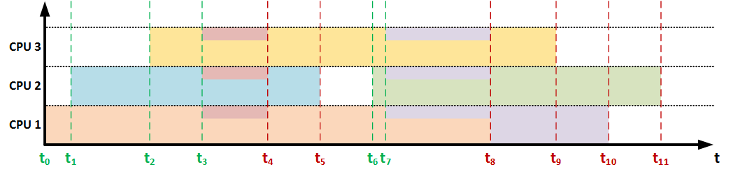
This approach is extremely understandable, however, when we speak about a pro-processor (multi-core) system, the situation becomes more complicated:
Analysis of these aspects showed that it is impossible to predict the execution time of the application in advance, but this value can be adjusted upon the occurrence of certain events affecting the current computing resource allocated for the calculations, followed by the issuance to the user. These events are: the arrival of a new task and the completion of the task being performed . It is upon the occurrence of these events that it is proposed to carry out a forecast correction.
It becomes clear that if any of these events occur, it is necessary to recalculate the allocated resource for each task (in cases with a known distribution of resources between tasks) or obtain this value in any way using the built-in (language or operating) tools, then recalculate the remaining time taking into account the allocated resource. But for this we need to know how much work has already been done by the process. Therefore, it is proposed to organize some storage (possibly a table in a DBMS), which will contain the necessary information, for example:
It is supposed to implement the following algorithm (metacode):
Conclusion: having an advance forecast for “ideal” conditions, we can practically “on the fly” correct the predicted percentage of “heavy” consecutive calculations when the load on the system changes and give the user these values upon request.
Specific implementations may have their own characteristics that complicate or simplify life, but the purpose of the article is not to analyze delicate cases, but only to offer the above approach to a fair trial of the reader (primarily on the subject of viability).
- receiving requests from users for some typical sequential "heavy" calculations;
- implementation of calculations;
- issuing information (on request) about the remaining computation time;
- issuing the results of calculations on their completion.
A number of circumstances should be clarified:
- By sequential calculation, we mean a calculation that is carried out by no more than one processor core (non-parallelizable process), since At this stage of creating the system, the task of parallelizing the calculations themselves is not worth it. In the future, the word "consistent" will be omitted;
- calculations are typical, i.e. the same algorithm is used for calculations, the execution time of which for a given computing system mainly depends on the dimension of the source data (the dimension is denoted by the number N), and not on their actual values;
- calculations are assumed to be predominantly “heavy”, which requires substantial time to complete (from seconds to hours and, possibly, more);
- It is assumed that the nature of the change in the intensity of applications for calculations and the corresponding values of the dimensions N are unknown.
The author’s initial attempts to predict the computation time had poor accuracy. For the "by eye" algorithm, the dependence of time on N was selected using power coefficients so as to minimize the average deviation. As a result of such test calculations, not very pleasant results were obtained:
| N | Real time (s) | Estimated time (sec) |
| 417 | 9.60 | 5.04 ± 0.96 |
| 689 | 26.20 | 18.33 ± 3.50 |
| 1165 | 78.40 | 70.56 ± 13.48 |
| 2049 | 264.60 | 300.34 ± 57.40 |
| 3001 | 654.20 | 799.24 ± 152.74 |
| 3341 | 875.80 | 1,052.50 ± 201.13 |
| 4769 | 2323.60 | 2,621.69 ± 501.01 |
| 5449 | 3424,10 | 3,690.10 ± 705.18 |
| 6129 | 4811.80 | 4,988.97 ± 953.40 |
To help, as often happens, came the classics. The words “interpolation” and “extrapolation”, long forgotten, were recalled, and searches on the Internet began in suspicion of the correctness of the chosen direction. A number of posts, articles and other resources were re-read. The main conclusion is as follows: to solve the problem of predicting the values of a certain unknown function of one variable, the Chebyshev or Lagrange polynomials are most often used. It turned out that it makes sense to use the Chebyshev polynomials (in principle, they could be replaced by the OLS) in cases where there is no confidence in the existing “argument-value” set, and Lagrange polynomials are good in the opposite case. The second looked like what was needed. Indeed, why not create “ideal” conditions for testing the computation algorithm on a specific system (select the core with a load of 100%) and not collect enough statistics to construct the Lagrange polynomial?
Graphic example of the construction of the Lagrange polynomial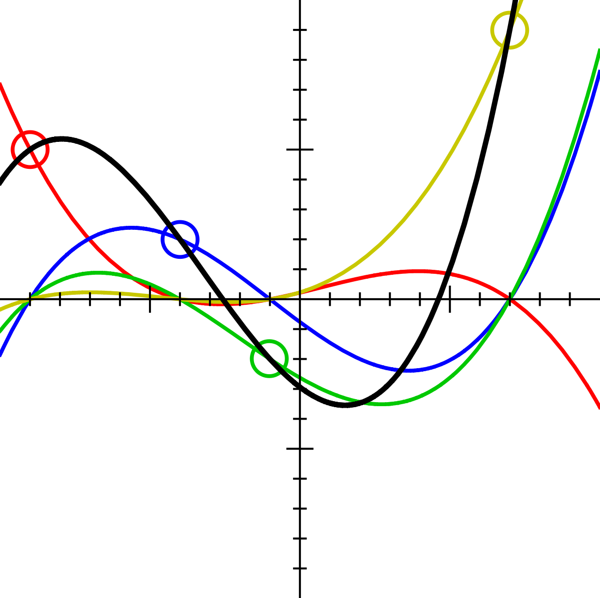
User Lagrange polynomial User: Acdx - Self-made, based on Image: Lagrangepolys.png . Under the license CC BY-SA 3.0 from Wikimedia Commons .
User Lagrange polynomial User: Acdx - Self-made, based on Image: Lagrangepolys.png . Under the license CC BY-SA 3.0 from Wikimedia Commons .
Meanwhile, there are already implemented algorithms for constructing the Lagrange polynomial, for example, here . The algorithm adapted for the task began to show similar (modulo deviations) results when extrapolating on an increasing set of statistics (for the forecast with N = 1165 real time was used with N = 417 and N = 689, for the forecast with N = 2049: N = 417, N = 689 and N = 1165, etc.):
| N | Real time (s) | Estimated time (sec) |
| 417 | 9.60 | - |
| 689 | 26.20 | - |
| 1165 | 78.40 | 55.25 |
| 2049 | 264.60 | 253.51 |
| 3001 | 654.20 | 617.72 |
| 3341 | 875.80 | 863.74 |
| 4769 | 2323.60 | 2899.77 |
| 5449 | 3424,10 | 2700.96 |
| 6129 | 4811.80 | 5862.79 |
When interpolating with the Lagrange polynomial, the results turned out to be impressive starting with N = 2049 (one sample was successively excluded from the sample and the calculation of the excluded measurement was made):
| N | Real time (s) | Estimated time (sec) |
| 417 | 9.60 | - |
| 689 | 26.20 | 2.58 |
| 1165 | 78.40 | 98.35 |
| 2049 | 264.60 | 245.74 |
| 3001 | 654.20 | 664.15 |
| 3341 | 875.80 | 862.91 |
| 4769 | 2323.60 | 2407.75 |
| 5449 | 3424,10 | 3251.71 |
| 6129 | 4811.80 | - |
Indeed, at N = 689 and N = 1165, the deviation of the predicted value from the real value was, respectively, about 90% and 25% , which is unacceptable, however, starting from N = 2049 and further the deviation was in the range of 1.5-7% , which can treat as a good result.
')
Polynomial: F (x) = -5.35771746746065e-22 * x ^ 7 + 1.23182612519573e-17 * x ^ 6 - 1.14069960055193e-13 * x ^ 5 + 5.44407657742344e-10 * x ^ 4 - 1.39944148088413e-6 * x ^ 3 + 0.00196094886960409 * x ^ 2 - 1.22001773413031 * x + 263.749105425487
The degree of the polynomial, if necessary, can be reduced to the desired one by easily changing the algorithm (in principle, for the author’s task it was possible to manage with the 3rd degree)
Graphs of this polynomial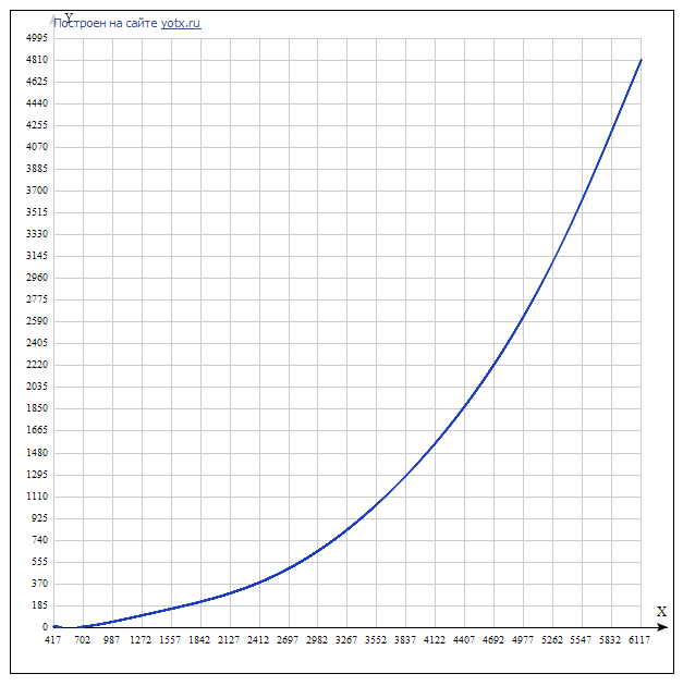
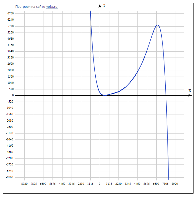
It is important to note that the polynomial is interpolation, and therefore, for values outside the [N min ; N max ] range, the quality of the forecast leaves much to be desired:
It is important to note that the polynomial is interpolation, and therefore, for values outside the [N min ; N max ] range, the quality of the forecast leaves much to be desired:
Conclusion: it makes sense to collect enough statistics in advance in “ideal” conditions (especially for large N values), to build the Lagrange polynomial and, upon receipt of applications, to obtain the forecast of the time of their calculations by substituting N i into the finished polynomial.
This approach is extremely understandable, however, when we speak about a pro-processor (multi-core) system, the situation becomes more complicated:
- Firstly, the above approach is suitable for cases where the number of applications (tasks) X <= Y, where Y is the number of cores. In other words, the system does nothing except calculations, and each task is provided with a 100% resource of the corresponding core.
- Secondly, when X> Y, the OS should divide the computational resource between tasks (for example, when manually launching tasks in Ubuntu server 14.04 through the screen, the computational resource is divided between tasks evenly according to the X / Y formula * 100%).
- Thirdly, the nature of the receipt of applications and the corresponding N values is not known in advance, which makes it impossible to predict the time for any distribution formula of the computing resource (for example, for the same X / Y * 100%).
Analysis of these aspects showed that it is impossible to predict the execution time of the application in advance, but this value can be adjusted upon the occurrence of certain events affecting the current computing resource allocated for the calculations, followed by the issuance to the user. These events are: the arrival of a new task and the completion of the task being performed . It is upon the occurrence of these events that it is proposed to carry out a forecast correction.
It becomes clear that if any of these events occur, it is necessary to recalculate the allocated resource for each task (in cases with a known distribution of resources between tasks) or obtain this value in any way using the built-in (language or operating) tools, then recalculate the remaining time taking into account the allocated resource. But for this we need to know how much work has already been done by the process. Therefore, it is proposed to organize some storage (possibly a table in a DBMS), which will contain the necessary information, for example:
| Task id | Start | the end | Lagrange (N) | Done | Last request | Last correction | Current CPU |
| 2457 | 12:46:11 | ... | Lagrange (N) | 0.45324 | ... | 12:46:45 | 1.00 |
| 6574 | 12:46:40 | ... | Lagrange (N) | 0.08399 | ... | 12:46:45 | 1.00 |
| 2623 | 12:44:23 | 12:46:45 | Lagrange (N) | 1.00 | ... | 12:46:45 | 0 |
| ... | ... | ... | ... | ... | ... | ... | ... |
It is supposed to implement the following algorithm (metacode):
- When a user has received a request about the status of the task:
- <Done> + = (<Request Time> - MAX (<Last Request>, <Last Correction>)) * <Current CPU> / <Lagrange (N)>;
- <Last request> = <Request moment>;
- Return to user <Done> and <Current CPU>.
- When a new task arrives:
- Create a new <task ID>;
- Record the start time at <Start>;
- Calculate and record the runtime forecast in “ideal” conditions in <Lagrange (N)>;
- <Done> = 0;
- <Last Request> = 00:00:00;
- Call the correction procedure.
- When the task is completed, you can delete the record altogether, but in any case, call the correction procedure.
- Correction procedure:
- For all records: <Last correction> = <Current time> (it makes sense to keep this value somewhere separate);
- Receive and record for each task the corresponding <Current CPU>.
Conclusion: having an advance forecast for “ideal” conditions, we can practically “on the fly” correct the predicted percentage of “heavy” consecutive calculations when the load on the system changes and give the user these values upon request.
Specific implementations may have their own characteristics that complicate or simplify life, but the purpose of the article is not to analyze delicate cases, but only to offer the above approach to a fair trial of the reader (primarily on the subject of viability).
Source: https://habr.com/ru/post/258791/
All Articles