Scala data analysis. We consider the correlation of the 21st century

It is very important to choose the right tool for data analysis. On the Kaggle.com forums, where international competitions in Data Science are held, people often ask which tool is better. The first lines of popularity are R and Python. In the article, we will talk about an alternative data analysis technology stack, made on the basis of the Scala programming language and the Spark distributed computing platform.

How did we come to this? In Retail Rocket, we do a lot of machine learning on very large amounts of data. Previously, for the development of prototypes, we used the IPython + Pyhs2 combination (hive driver for Python) + Pandas + Sklearn. At the end of the summer of 2014, we made a fundamental decision to switch to Spark , since the experiments showed that we would get a 3-4 fold increase in performance on the same server park.

Another plus is that we can use one programming language for modeling and code that will work on the combat servers. For us, this was a great advantage, because before that we used 4 languages ​​simultaneously: Hive, Pig, Java, Python, for a small team this is a serious problem.

Spark well supports working with Python / Scala / Java through an API. We decided to choose Scala, since Spark was written on it, that is, it is possible to analyze its source code and, if necessary, correct errors, plus - this is the JVM on which the whole Hadoop is running. Analysis of the programming language forums under Spark reduced to the following:
')
Scala:
+ functional;
+ native to Spark;
+ works on JVM, which means native to Hadoop;
+ strict static typing;
- rather complicated input, but the code is readable.

Python:
+ popular;
+ simple;
- dynamic typing;
- performance is worse than Scala.

Java:
+ popularity;
+ native to Hadoop;
- too much code.

More details on the choice of programming language for Spark can be found here .

I must say that the choice was not easy, because at that moment no one in the team knew Scala.
A well-known fact: to learn how to communicate well in a language, you need to immerse yourself in the language environment and use it as often as possible. Therefore, for modeling and quick data analysis, we abandoned the Python stack in favor of Scala.

The first step was to find a replacement for IPython, the options were as follows:
1) Zeppelin - an IPython-like notebook for Spark;
2) ISpark;
3) Spark Notebook;
4) Spark IPython Notebook from IBM .

So far, the choice has fallen on ISpark, since it is simple - this is IPython for Scala / Spark, it was relatively easy to attach HighCharts and R charts to it. And we didn’t have any problems connecting it to the Yarn cluster.

Our story about the Scala data analysis environment consists of three parts:
1) A simple task on Scala in ISpark, which will be executed locally on Spark.
2) Setup and installation of components for work in ISpark.
3) We write Machine Learning task on Scala, using libraries R.
And if this article is popular, I will write two others. ;)

Task

Let's try to answer the question: does the average purchase check in the online store depend on the client’s static parameters, which include the settlement, browser type (mobile / Desktop), operating system and browser version? This can be done with the help of Mutual Information.

In Retail Rocket, we use entropy much where we use our recommender algorithms and analysis: the classical Shannon formula, the Kullback-Leibler discrepancy, mutual information. We even applied for a report on the RecSys conference on this topic. These measures are devoted to a separate, albeit small, section in the well-known textbook on machine learning, Murphy.

Let's analyze on real data Retail Rocket . Previously, I copied the sample from our cluster to my computer as a csv file.

Data loading

Here we use ISpark and Spark, running in local mode, that is, all calculations occur locally, the distribution goes to the cores. Actually everything is written in the comments. Most importantly, at the output we get RDD (Spark data structure), which is a collection of case classes of type Row, which is defined in the code. This will allow access to the fields via ".", For example _.categoryId.

At the entrance:

import org.apache.spark.rdd.RDD import org.apache.spark.sql._ import org.tribbloid.ispark.display.dsl._ import scala.util.Try val sqlContext = new org.apache.spark.sql.SQLContext(sc) import sqlContext.implicits._ //  CASE class,     dataframe case class Row(categoryId: Long, orderId: String ,cityId: String, osName: String, osFamily: String, uaType: String, uaName: String,aov: Double) //     val   sc (Spark Context),   Ipython  val aov = sc.textFile("file:///Users/rzykov/Downloads/AOVC.csv") //   val dataAov = aov.flatMap { line => Try { line.split(",") match { case Array(categoryId, orderId, cityId, osName, osFamily, uaType, uaName, aov) => Row(categoryId.toLong + 100, orderId, cityId, osName, osFamily, osFamily, uaType, aov.toDouble) } }.toOption } 

At the exit:

 MapPartitionsRDD[4] at map at <console>:28 

Now look at the data itself:

This line uses the new DataFrame data type added in Spark in version 1.3.0, it is very similar to the similar structure in the pandas library in Python. toDf picks up our case class Row, thanks to which it gets the names of the fields and their types.

For further analysis, you need to select any one category, preferably with a large amount of data. For this you need to get a list of the most popular categories.

At the entrance:

 //   dataAov.map { x => x.categoryId } //   categoryId .countByValue() //     categoryId .toSeq .sortBy( - _._2) //       .take(10) //   10  

At the output we got an array of tuples (tuple) in the format (categoryId, frequency):

 ArrayBuffer((314,3068), (132,2229), (128,1770), (270,1483), (139,1379), (107,1366), (177,1311), (226,1268), (103,1259), (127,1204)) 

For further work, I decided to choose the 128th category.

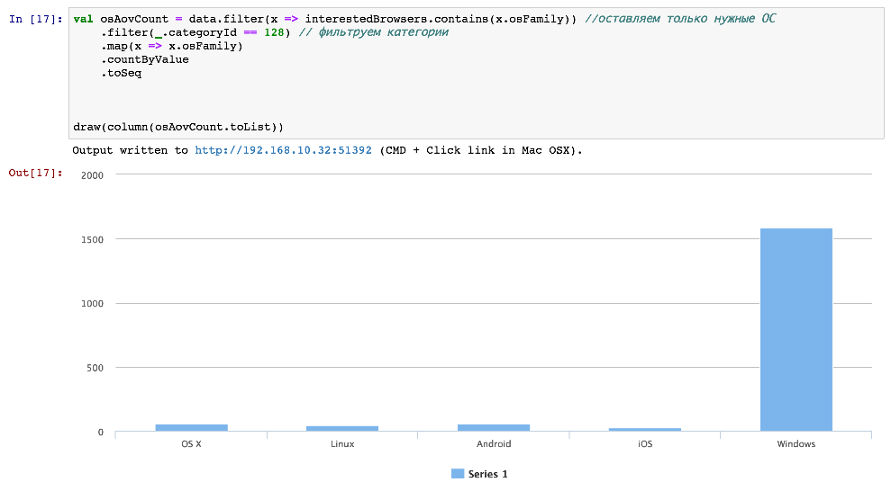
Prepare the data: filter the necessary types of operating systems so as not to litter the graphics with garbage.

At the entrance:

 val interestedBrowsers = List("Android", "OS X", "iOS", "Linux", "Windows") val osAov = dataAov.filter(x => interestedBrowsers.contains(x.osFamily)) //    .filter(_.categoryId == 128) //   .map(x => (x.osFamily, (x.aov, 1.0))) //      .reduceByKey((x, y) => (x._1 + y._1, x._2 + y._2)) .map{ case(osFamily, (revenue, orders)) => (osFamily, revenue/orders) } .collect() 

At the output, an array of tuples (tuple) in OS format, average check:

 Array((OS X,4859.827586206897), (Linux,3730.4347826086955), (iOS,3964.6153846153848), (Android,3670.8474576271187), (Windows,3261.030993042378)) 

I want to render, let's do it in HighCharts:

Theoretically, you can use any HighCharts graphics if they are supported in Wisp . All graphics are interactive.

Let's try to do the same, but through R.
Run R client:

 import org.ddahl.rscala._ import ru.retailrocket.ispark._ def connect() = RClient("R", false) @transient val r = connect() 

We build the schedule itself:

So you can build any R graphics right in your IPython notepad.

Mutual Information

The graphs show that there is a dependency, but will this metric confirm us? There are many ways to do this. In our case, we use mutual information ( Mutual Information ) between the values ​​in the table. It measures the mutual dependence between the distributions of two random (discrete) quantities.

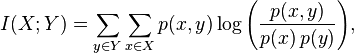
For discrete distributions, it is calculated by the formula:



But we are interested in a more practical metric: Maximal Information Coefficient (MIC), for the calculation of which for continuous variables one has to go for tricks. This is how the definition of this parameter sounds.

Let D = (x, y) be a set of n ordered pairs of elements of random variables X and Y. This two-dimensional space is divided into X and Y grids, grouping the values ​​of x and y into X and Y tilings, respectively (recall the histograms!).



where B (n) is the size of the grid, I ∗ (D, X, Y) is mutual information on splitting X and Y. The denominator indicates the logarithm, which serves to normalize the MIC to the values ​​of the interval [0, 1]. MIC takes continuous values ​​in the interval [0,1]: for extreme values ​​it is equal to 1, if the dependence is, 0 - if it is not. What else you can read on this topic is listed at the end of the article, in the list of references.

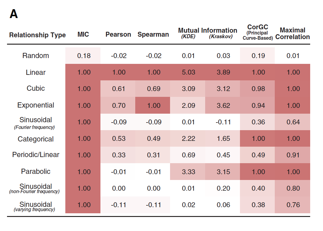
The book MIC (mutual information) is called the correlation of the 21st century. And that's why! The graph below shows 6 dependencies (graphs C - H). For them, the Pearson and MIC correlations were calculated, they are marked with the corresponding letters in the graph on the left. As we see, the Pearson correlation is almost zero, while the MIC shows the dependence (graphs F, G, E).

Original source: people.cs.ubc.ca

The table below shows a number of metrics that were calculated on different dependencies: random, linear, cubic, etc. The table shows that MIC behaves very well, detecting non-linear dependencies:


Another interesting graph illustrates the effects of noise on the MIC:


In our case, we are dealing with the calculation of MIC, when the variable Aov is continuous and all others are discrete with unordered values, for example, the type of browser. To correctly calculate the MIC, you will need the discretization of the variable Aov. We will use a ready-made solution from the site exploredata.net . There is one problem with this solution: it considers that both variables are continuous and expressed in Float values. Therefore, we will have to trick the code by encoding the values ​​of discrete values ​​in Float and randomly changing the order of these values. To do this, you will have to do a lot of iterations with random order (we will do 100), and as a result we will take the maximum MIC value.

 import data.VarPairData import mine.core.MineParameters import analysis.Analysis import analysis.results.BriefResult import scala.util.Random //  ,    "" def encode(col: Array[String]): Array[Double] = { val ns = scala.util.Random.shuffle(1 to col.toSet.size) val encMap = col.toSet.zip(ns).toMap col.map{encMap(_).toDouble} } //   MIC def mic(x: Array[Double], y: Array[Double]) = { val data = new VarPairData(x.map(_.toFloat), y.map(_.toFloat)) val params = new MineParameters(0.6.toFloat, 15, 0, null) val res = Analysis.getResult(classOf[BriefResult], data, params) res.getMIC } //          def micMax(x: Array[Double], y: Array[Double], n: Int = 100) = (for{ i <- 1 to 100} yield mic(x, y)).max 

Well, we are close to the finals, now let's do the calculation:

 val aov = dataAov.filter(x => interestedBrowsers.contains(x.osFamily)) //    .filter(_.categoryId == 128) //   //osFamily var aovMic = aov.map(x => (x.osFamily, x.aov)).collect() println("osFamily MIC =" + micMax(encode(aovMic.map(_._1)), aovMic.map(_._2))) //orderId aovMic = aov.map(x => (x.orderId, x.aov)).collect() println("orderId MIC =" + micMax(encode(aovMic.map(_._1)), aovMic.map(_._2))) //cityId aovMic = aov.map(x => (x.cityId, x.aov)).collect() println("cityId MIC =" + micMax(encode(aovMic.map(_._1)), aovMic.map(_._2))) //uaName aovMic = aov.map(x => (x.uaName, x.aov)).collect() println("uaName MIC =" + mic(encode(aovMic.map(_._1)), aovMic.map(_._2))) //aov println("aov MIC =" + micMax(aovMic.map(_._2), aovMic.map(_._2))) //random println("random MIC =" + mic(aovMic.map(_ => math.random*100.0), aovMic.map(_._2))) 

At the exit:

 osFamily MIC =0.06658 orderId MIC =0.10074 cityId MIC =0.07281 aov MIC =0.99999 uaName MIC =0.05297 random MIC =0.10599 

For the experiment, I added a random variable with a uniform distribution and AOV itself.
As we see, almost all MICs are below a random variable (random MIC), which can be considered the “conditional” decision threshold. Aov MIC is almost equal to one, which is natural, since the correlation to itself is equal to 1.

An interesting question arises: why do we see the dependence in the graphs, and the MIC is zero? You can come up with many hypotheses, but most likely for the case of os Family everything is pretty simple - the number of Windows machines far exceeds the number of others:

Conclusion

I hope that Scala will get its popularity among data analysts (Data Scientists). This is very convenient, since it is possible to work with the standard IPython notebook + to get all the features of Spark. This code can easily work with terabyte data arrays, for this you just need to change the configuration line in ISpark, specifying the URI of your cluster.

By the way, we have open vacancies in this area:

• Junior Analyst
• Research analyst

Useful links:
Scientific article, on the basis of which MIC was developed .
Note on KDnuggets about mutual information (there is a video).
C library for calculating MIC with wrappers for Python and MATLAB / OCTAVE .
The site of the author of a scientific article that developed MIC (there is a module for R and a Java library on the site ).