Simple suffix tree

Suffix tree is a powerful structure that allows you to unexpectedly effectively solve myriads of complex search tasks on unstructured data arrays. Unfortunately, the known algorithms for constructing a suffix tree (mainly the algorithm proposed by Esko Ukkonen) are quite difficult to understand and time-consuming to implement. Only relatively recently, in 2011, by the efforts of Dany Breslauer and Giuseppe Italiano, a relatively simple construction method was invented, which is in fact a simplified version of Peter Weiner’s algorithm, who invented suffix trees in 1973 . If you do not know what a suffix tree is or have always been afraid of it, then this is your chance to study it and at the same time master a relatively simple way of building it.

Before proceeding to the description of the suffix tree, we define the terminology. The input for the algorithm is the string s, consisting of n characters s [0], s [1], ..., s [n-1]. Each character is a byte. Although, of course, everything described here will work for any other sequences: bits, two-byte Unicode characters, two-bit characters of DNA sequences, and so on. Additionally, we assume that s [n-1] is equal to the symbol 0, which is not found anywhere else in s. This last restriction serves only to simplify the narrative and, in fact, it is enough to just get rid of it. Lines of the form s [i..j] = s [i] s [i + 1] ... s [j], where i and j are some whole numbers, are called, as usual, substrings. Substrings of the form s [i..n-1], where i is some integer, are called suffixes.

So, the main character. The suffix tree for string s is the minimum in the number of vertices tree, each edge of which is marked by a non-empty substring s in such a way that each suffix s [i..n-1] can be read from the root to any leaf and, vice versa , each line read on the way from the root to any sheet is a suffix s. The easiest way to deal with this definition is an example (disregard, for now, pos, len and to):


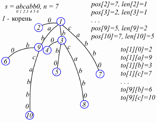
In a suffix tree no more than 2n + 1 vertices. This can be seen if the tree is constructed by successively inserting suffixes: when inserting the next suffix, a new leaf may appear and the vertex to which this leaf is attached. Since s [n-1] is a special symbol, there are exactly n leaves in the suffix tree. Vertices will be numbered with integers. We will store the father of the vertex v in par [v]. The label on the edge from v to father v is stored as a pair of numbers: the length of the label len [v] and the position pos [v] immediately after this label in s, i.e. if the label is a string t, then t = s [pos [v] -len [v] .. pos [v] -1]. Let some vertex v have k children and t ₁ , t ₂ , ..., t _k are labels on edges from v to children. Note that the first characters of the strings t ₁ , t ₂ , ..., t _k are pairwise different, which means that references to the children v can be stored in the map to [v], which displays the first character of the label in the corresponding offspring. I will avoid the object-oriented approach in the description of structures, in order to make the code shorter and you think “Wow, what a compact code”. So, the suffix tree is represented as follows (now you can pay attention to pos, len, and to in the figure above):

int sz; //    int pos[0..sz-1], len[0..sz-1], par[0..sz-1]; //par[v] –   v std::map<char, int> to[0..sz-1]; //to[v] –     v 

The first important property is that the suffix tree occupies O (n) memory.
')
The string written on the path from the root to the vertex v will be denoted by str (v); str (v) is used only in reasoning and is not explicitly stored anywhere.

Suffix Tree Usage Examples

To get comfortable with the suffix tree and at the same time understand how to use it, consider a few examples.

Search for substrings in s

Perhaps the very first thing that comes to mind is to use the suffix tree to search for substrings. It is quite simple to note that the string u is a substring of the string s if and only if u can be read from the root of the suffix tree (since u = s [i..j] for some i and j and therefore the suffix s [i. .n-1] starts with u).

The number of different substrings in the string s

By the same reasoning, it can be established that each substring s corresponds to a certain position on the label of some edge of the suffix tree. The number of different substrings is the number of such positions and it is equal to the sum of len [v] over all vertices v except the root.

Data compression LZ77

The example is more complicated. The idea of ​​compressing LZ77 (google Lempel, Ziv) is simple and can be described with the following pseudo code:

 for (int i = 0; i < n; i = j+1) //  s[0..n-1] if ( s[i]     s[0..i-1]) { j = i,      s[i]; //      } else { j = max{j    d < i ,  s[i..j] = s[d..d+ji]}; d =  0,1,…,i-1 ,  s[d..d+ji] = s[i..j];       (j-i+1, id) //      } } 

For example, the string “aababababaaab” will be encoded as “a (1,1) b (7,2) (3,10)” (note the “overlapping” of abababa strings). Of course, implementation details can be very different, but the basic idea is used in many compression algorithms. With the help of the suffix tree, you can compress s in a similar way for O (n). To do this, we supplement each vertex v of our tree with a field start [v] such that start [v] is equal to the smallest p for which s [p..p + | str (v) | -1] = str (v), where | str (v) | Is the length of str (v). It is clear that for leaves this value is easily calculated. For the remaining vertices, the start field is calculated by a single depth traverse, start [v] = min {start [v ₁ ], start [v ₂ ], ..., start [v _k ]}, where v ₁ , v ₂ , ..., v _k are children of v. Now, to calculate the next value of j in our compression algorithm, it is enough to read the string s [i..n-1] from the root as long as the current vertex v in the tree has start [v] <i; d can be chosen equal to the last such value of start [v].

Building a suffix tree

I warn you in advance that, despite the fact that Weiner's simplified algorithm is simpler than Ukkonen’s algorithm and Weiner's classical algorithm, it is nevertheless still a non-trivial algorithm, and you need to make some efforts to understand it.

Overall plan. Prefix links

The algorithm starts from an empty tree and sequentially adds the suffixes s [n-1..n-1], s [n-2..n-1], ..., s [0..n-1] (just in case I’ll make a reservation that in the implementation under discussion, the extend function works correctly only if suffixes are added exactly in the order of increasing lengths, starting with the shortest; that is, for example, the code “for (int i = n-3; i> = 0; i--) extend (i) "contains a bug):

 for (int i = n-1; i >= 0; i--) extend(i); //    s[i..n-1] 

Thus, at the kth loop iteration, we have a suffix tree for the string s [n-k + 1..n-1] and add the suffix s [nk..n-1] to the tree. It is clear that adding a new longest suffix requires inserting one new sheet and, possibly, one new vertex that “breaks” the old edge. The main problem is to find a position in the tree where a new leaf will be attached. To solve this problem, the suffix tree is supplemented with prefix links .

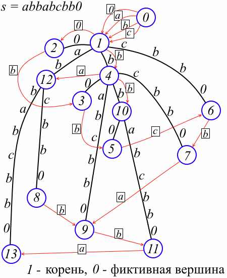
With each vertex v, we associate prefix links link [v] - a map that maps characters to vertex numbers as follows: for the character a, link [v] [a] is defined if and only if there is a vertex w in the tree such that str ( w) = a str (v) and in this case link [v] [a] = w. (If you were familiar with the classical Weiner algorithm, you noticed that our prefix links correspond to the “explicit” classical prefix links, and the “implicit” links, it turns out, are not required at all; if you were familiar with the Ukkonen algorithm, you might notice that The prefix links are reversed “suffix links.”) In the figure, the prefix links are marked in red, and the symbols corresponding to the links are written in rectangles (see below for the dummy vertex 0).


Thus, we have an additional structure:

 std::map<char, int> link[0..sz-1]; //  

By definition, at each vertex there can be at most one prefix link, from which we conclude that the link occupies O (n) memory.

We first agree on the technical nuance of the implementation presented here. The root of the tree is vertex 1, and 0 is a dummy vertex such that link [0] [a] = 1 for all characters a; in addition, par [1] = 0 and len [1] = 1. The dummy vertex does not carry a special semantic load, but allows one to handle certain special cases uniformly. Below this will be explained in more detail, but for now do not pay attention to it. Let us proceed to the description of the algorithm for inserting a new suffix.

Algorithm

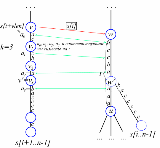
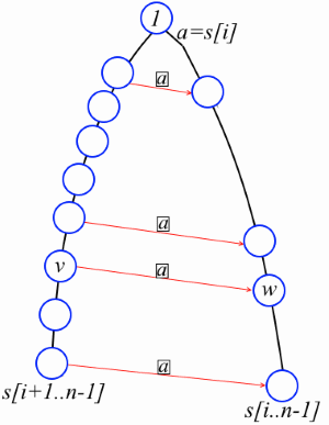Lemma. Let i be some number from 0 to n-2. Consider the suffix tree of the string s [k..n-1], where k <= i. If w is a non-root vertex on the path from the root to the leaf corresponding to s [i..n-1], then on the path from the root to the leaf corresponding to s [i + 1..n-1] there is a vertex v such that s [i] str (v) = str (w) and link [v] [s [i]] = w (see figure).

Let's prove it. Denote str (w) = s [i] t. By definition of a suffix tree, either w is a leaf, or w has at least two descendants. If w is a leaf, then v is the leaf corresponding to the string s [i + 1..n-1]. Let w not be a leaf. Then there are some different characters a and b such that to [w] [a] leads to one child w, and to [w] [b] to another. So s [i] ta and s [i] tb are substrings of s (at least one of them starts not in position i). Therefore, ta and tb are also substrings and there must be a vertex v in the tree such that str (v) = t. It is clear that v lies on the path to the leaf corresponding to s [i + 1..n-1], and, by the definition of prefix links, we have link [v] [s [i]] = w.

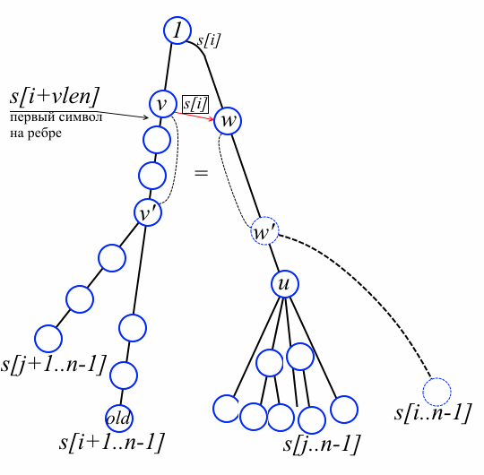
So, we suppose we have a suffix tree for the string s [i + 1..n-1] and are going to add a sheet for the string s [i..n-1] and accordingly update the prefix links. See picture below. Denote by old the sheet corresponding to s [i + 1..n-1]. The “docking” place of the new sheet is the vertex w ', which may not yet have been created. W denotes a vertex immediately above w '(if w' is already in the tree, then w = w 'and in this case it is enough to add a new leaf). For simplicity, we first consider the case when w is not a root. By the lemma, there is a vertex v on the path from old to the root such that link [v] [s [i]] = w.


Fact 1. On the way from v to old there are no vertices v "such that link [v"] [s [i]] is defined. Suppose by contradiction, v "is such a vertex. Then the link [v ''] [s [i]] vertex is the ancestor of w 'and, simultaneously, the descendant of w (by the definition of prefix links). But we chose w as the nearest vertex from the docking point! Contradiction.

Our algorithm first finds v and w. At the same time, we calculate the value of | str (v) | +1 in the vlen variable and add all the passed vertices to the stack of the path — they will still be useful. Note that at the end of the cycle, s [i + vlen] is equal to the first character on the edge from v to scion v on the path to old (see figure above).

  int v, vlen = n - i, old = sz – 1;//   old –    for (v = old; !link[v].count(s[i]); v = par[v]) { vlen -= len[v]; path.push(v); } int w = link[v][s[i]]; 

Fact 2. A vertex w 'is already present in the tree if and only if to [w] [s [i + vlen]] is not defined; in this case w = w '. If you meditate a little over the figure above and note about the meaning of the symbol s [i + vlen], this statement becomes obvious.

Fact 3. On the way from v to old, there is a vertex v 'such that s [i] str (v') = str (w '), even if w' does not yet exist. If w 'is already in the tree, then the statement is obvious in fact 2 and v' = v. Suppose w 'has yet to be created. Let u = to [w] [s [i + vlen]]. Choose an arbitrary leaf from the subtree with root u; Let this sheet correspond to the suffix s [j..n-1] for some j. The not yet inserted suffix s [i..n-1] and the suffix s [j..n-1] diverge at the “implicit” vertex w '. But the leaves corresponding to s [j + 1..n-1] and s [i + 1..n-1] are already represented in the tree and diverge at some vertex v '. It is clear that s [i] str (v ') = str (w'), which means v 'lies on the path from v to old. This is the place to look at the picture above for the last time. We proceed to the main part of the algorithm.

Now that we have found w, our task is to find a place for joining a new sheet, i.e. in fact, we are looking for len [w '] and vertex v'. In the case w = w ', it suffices to attach the sheet to w and draw a prefix reference from old to this sheet. Consider the complex case when w! = W ', i.e. is an edge from w by the symbol s [i + vlen]. Denote, again, u = to [w] [s [i + vlen]]. We successively get the vertices from the stack of the path until we find a vertex v 'such that s [i] str (v') = str (w '). How do we determine that we have found the right vertex? Let v ₁ , v ₂ , ..., v _k - the top vertices from the stack stack and v _k = v '(see the figure below). Let a _p denote the first character on the edge that follows from v _p to the descendant v _p on the path to old. We define a ₀ = s [i + vlen]. Let t be a label on an edge from w to u. The symbol t [len [v ₁ ] + len [v ₂ ] + ... + len [v _p -1]] will be called the symbol corresponding to a _p on t. Since w 'is the branch point of the suffix s [i..n-1] on the edge from w to u, the symbol a _{k is} not equal to the corresponding symbol on t. On the other hand, for the same reason, for each p = 0,1, ..., k-1, the symbol a _p is equal to the corresponding symbol on t. With the picture this reasoning will be clearer:



This comment is the core of Weiner's simplified algorithm. Interestingly, it is enough for us to compare only the first symbol on the edges with the corresponding symbol on t, and not all symbols. In essence, this simple observation is what Breslauer and Italiano noticed, and for some reason nobody noticed before. It remains to remember to draw a prefix reference from v 'to w' and a prefix reference from old to a new sheet. So, the algorithm inserts a new suffix s [i..n-1] as follows:

  if (to[w].count(s[i + vlen])) { // w != w' int u = to[w][s[i + vlen]]; //sz –    w',    //.. w!=w',  s[pos[u] - len[u]] == s[i + vlen]      for (pos[sz] = pos[u] - len[u]; s[pos[sz]] == s[i + vlen]; pos[sz] += len[v]) { v = path.top(); path.pop(); //   v' vlen += len[v]; }    w  u  w'=sz; len[w'] = len[u]-(pos[u]-pos[sz]) link[v][s[i]] = sz; //   v'  w' w = sz++; // w = w'     } //    w  w' link[old][s[i]] = sz; //   old    sz   sz  w; len[sz] = n – (i + vlen) pos[sz++] = n; //pos     n 

It remains to consider the special case when w is the root. This situation is completely similar, but some values ​​are shifted by one. It would be possible, of course, to handle this case separately, but with the help of a fictitious vertex, it would be easier to make this and no additional code would be written. In this place, the important role is played by the fact that par [1] = 0, len [1] = 1 and link [0] [a] = 1 for all characters a. Thus, the cycle of searching for the vertex v will necessarily terminate at the vertex 0, and the value len [1] = 1 will provide the necessary shift by one. To understand the details is not difficult and I will leave it as an exercise. I hope the secret meaning of the fictitious peak on this should be clarified. Combining everything together, we get this solution:

 void attach(int child, int parent, char c, int child_len) //  { to[parent][c] = child; len[child] = child_len; par[child] = parent; } void extend(int i) //  ;   i=n-1,n-2,...,0 { int v, vlen = n - i, old = sz - 1; for (v = old; !link[v].count(s[i]); v = par[v]) { vlen -= len[v]; path.push(v); } //   vlen = |str(v)|+1 int w = link[v][s[i]]; if (to[w].count(s[i + vlen])) { // w != w' int u = to[w][s[i + vlen]]; for (pos[sz] = pos[u]-len[u]; s[pos[sz]]==s[i + vlen]; pos[sz] += len[v]) { v = path.top(); path.pop(); //   v' vlen += len[v]; } attach(sz, w, s[pos[u] - len[u]], len[u] - (pos[u] - pos[sz])); // w'(=sz)  w attach(u, sz, s[pos[sz]], pos[u] - pos[sz]); // u  w'(=sz) w = link[v][s[i]] = sz++; //    v'  w';  w = w'     } //    w   w' link[old][s[i]] = sz; //       attach(sz, w, s[i + vlen], n - (i + vlen)); //   sz   w' pos[sz++] = n; //pos     n } void init() { len[1] = 1; pos[1] = -1; par[1] = 0; //,  par[1] = 0  len[1] = 1 (!) for (int c = 0; c < 256; c++) link[0][c] = 1;//  0         } 

Evaluation of the time of the algorithm

In conclusion, let us understand why the whole described construction performs O (n) operations. The height of a vertex v is the number of vertices on the path from the root to v. Let me remind you that the step of the algorithm is the addition of a new suffix to the tree. Denote by h _{i the} height of the vertex corresponding to the longest suffix at the ith step. Let k _i be the number of vertices traversed from old to v at the ith step. How does the value of h _i change? If you take another look at the drawing to the lemma, having thought it over, you will notice that h _i <h _i-1 - k _i-1 + 2. The number of operations performed on the i-th step is proportional to k _i , which means, as we only what you noticed, O (h _{i + 1} - h _i + 2). From this it is obvious that the algorithm performs O (2n + (h ₁ - h ₂ ) + (h ₂ - h ₃ ) + ... + (h _n-1 - h _n )) = O (n) operations in the sum.

A small optimization note. Considering the access time to the maps, the Weiner algorithm's running time (as well as Ukkonen) is O (n log m), where m is the number of different characters in the string. When the alphabet is very small, instead of maps, it is better to use arrays to make Weiner truly linear.

To be fair, it should be noted that Weiner's simplified algorithm (and the classical even more so) consumes about one and a half to two times more memory than Ukkonen. Also, tests showed that the simplified Weiner works about 1.2 times slower (here it is slightly inferior to Ukkonen). Nevertheless, all these shortcomings are partly compensated by the simplicity of Weiner's implementation and the lack of a large number of pitfalls.

References in chronological order

P. Weiner. “Linear pattern matching algorithms” 1973 is Weiner's first article in which a suffix tree is entered and a linear algorithm is given.

E. McCreight. “A space economical suffix tree construction algorithm” 1976 is a more lightweight suffix tree construction algorithm.

E. Ukkonen. “On-line construction of suffix trees” 1995 - modification of the McCreit algorithm; most popular modern algorithm.

D. Breslauer, G. Italiano. “Near real-time suffix tree construction through the fringe marked ancestor problem” 2013 (preliminary version in 2011) - the description of Weiner's simplified algorithm in this article takes one paragraph (remark on the 10th page), and everything else is devoted to another close problem.

PS Thanks to Misha Rubinchik and Oleg Merkuryev for their help in testing the algorithm and suggestions for improving the code.

PPS In conclusion I cite