Multiklet R1 - the first tests
Time passes, and the multicellular processor continues to grow, develop. So far, however, does not multiply, and consists of only 4 cells, but this is all ahead of him. In this article I will try to describe the main features of the new Multiklet R1 processor, its characteristics and functionality, as well as compare the new generation processor with the dynasty's ancestor - the Multiklet P1 processor.
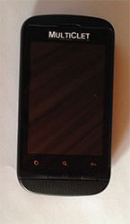
Let us briefly go over the historical issues of processor production, look briefly at the theoretical basis of our processors, pay attention to the features of the new processor and its main features, compare the P1 and R1 processors, show the prototype of the first product on R1, and finally make a small announcement.

Figure 1. Silicon wafer R1 processors
1. History of creation
Multiklet company was founded in 2010. Taking into account the developments of the synagogue project of the Ural architectural laboratory, which had been conducted since 2001 under the direction of NV Streltsov, a step was taken to create the first processor with the new Russian architecture. And all efforts resulted in the first representative of the universal multicellular architecture - the processor Multiklet P1. The letter “P” means aimed at performance (Performance). After the release of the processor, two versions of the debug kits were made, and then several serial devices, including a foaming machine, a Key_P1 data protection device. There was an active work of users, those who were interested to try something new. The result of this activity were examples of working with a touchscreen, asynchronous motor control, altimeter, three-axis sensor analyzer and more.
But, undoubtedly, it was necessary to rise to a new level. And in 2014, a dynamic reconfiguration processor called R1-1 was born. According to the test results, this revision went into prototypes, and the R1 processor, which has been available in a plastic case since March 2015, was released in December 2014. It is this processor that will be discussed in this article.
I will add that multicellular processors are being developed in Yekaterinburg, the crystal is baked in Malaysia at the SilTerra factory.
')
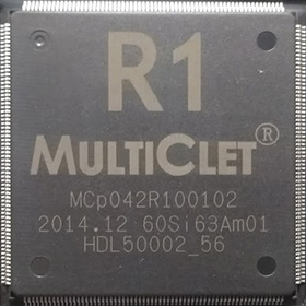
Figure 2. R1 processor
2. Brief fundamentals of architecture
The R1 processor, as well as the first representative of the multicellular architecture, consists of four cells. The architecture has the following basic principles:
Consider the composition of the processor unit - cells. The R1 processor cell contains a command selection and distribution unit (IDU), a control unit and a command decoder (CU), a buffer device (BUF), a switching device (SU), a result multiplexer, an interrupt controller (IC), a debugging unit (JTAG -GPR), a block of general-purpose registers (GPR), an actuator (EU) consisting of a double-precision arithmetic logic unit (hereinafter referred to as ALU) with a floating point (ALU_FLOAT), ALU for integers (ALU_INTEGER) and a block of data memory access (DMS).
The connecting element of cells is the extracellular environment, which is a wire connecting the switching devices of the cells and their inputs, outputs. The repository of results is the switch (SU), which stores information coming from the “intercellular environment”.
The main advantages of the architecture are low power consumption, achieving maximum performance, and dynamic resource allocation.
Low power consumption is achieved due to the simplicity of the implementation of this architecture, the use of the principle of broadcasting, the absence of complex blocks of transition predictors, cache, reordering of instructions, etc.
High performance is achieved due to the fact that “on direct” multicellular architecture is faster, and on “turns” it is not worse than existing architectures.
The whole program is a set of instructions, combined in paragraphs.
The paragraph of the multicellular architecture can be represented as a large command for a conventional processor architecture. A paragraph is meant by "direct", and transitions between paragraphs are "turns."

Figure 3. Turning illustration
If we briefly cover the advantages of the architecture, then with minor corrections I will quote the user AlexDi from the ixbt forum:
"Extraordinary execution of up to 4 arbitrary commands per clock, with an extraordinary depth of up to 64 commands, prediction of the transition long before the transition itself, pre-decoding of commands after the transition point, saving arithmetic flags for the results of all instructions."
Up to 12 commands can be sent for each execution (4 cells with three independent ports for ALU_FLOAT, ALU_INTEGER, DMS in each), but they have only one output, therefore, up to 4 commands can output the result in the current implementation of the architecture . The performance in Gigaflops is obtained at the peak due to the rate of execution of commands for complex multiplication of two arguments (a + bi) * (c + di), as a result we get 6 operations per cell, multiply by 4 cells and we get 24 operations per clock. Multiplying the number of operations per clock per frequency (for R1 is 100 MHz) we get 2.4 GFlops.
You can learn more about the architecture in the article “A multicellular processor is what?”
3. What's new in processor R1
Initially, it was supposed to slightly refine the P1 processor, but in the process of refinement, the R1 turned out to be almost completely new core. Now the program memory is common to all cells, the sampling mechanism has changed accordingly (in P1, each cell had its own program memory), and the mechanism for the distribution of results changed. Indirect addressing appeared, direct read and write commands were added (bypassing the queuing mechanism), work with index registers was improved. And most importantly, reconfiguration (the ability of cells to form groups) appeared.
The range of assembler commands has increased, a DTC memory unit has appeared. Quartz at 8-12 MHz is enough for clocking, it is possible to work with external memory such as SRAM, SDRAM, PROM, I / O. USB is now standard 2.0 device, RTC with calendar on board. And an important step was the operation of the analog block, the R1 processor contains 8 independent channels of delta-sigma ADC of 16 bits, 48 kilo samples per second and 1 DAC channel up to 100 megabytes per second (works at the system frequency). Initially it was planned that there would be two D / C channels, but one fully working D / A channel turned out.
Consider a little more detail a few innovations in the processor R1. But first, let me remind you what an example of a paragraph in assembly language looks like (for P1 and R1, you can write in C):
, . .
:
#0 0x10, 0x50 rdl 0x50, 0x12345. .
- , , , .
, , , . ge lt .
:
1) : ge ARG1, ARG2 — « »
: «1» ARG1 >= ARG2, 0
2) : lt ARG1, ARG2 — «»
: «1» ARG1 < ARG2, 0
0 3, 4 10, 11 . , :
, DFADDR, , , switch-case. :
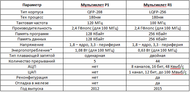
4. P1 R1
. P1 80, 100 120 . R1 PLL 8-12 .
P1 , . R1 , SRAM, SDRAM I/O. R1 .
, , R1 DTC, . R1, P1, .
R1 512 . P1 128 , 128 .
. , R1 .
, R1 – , .. . , , , , « » , 3 , . , , , fork() , , :
3 , main():
main1(), main2(), main3(), :
P1 R1:
* 75% DMAC + 25% ADD. R1 FFT 1,05 . P1 .
R1 clock gating , R1 1,5 P1.
, , . Geany.
Windows Linux. .
5.
, R1 , , , . 4. 5.
4.
5.
( ) , .
, :
, .
!
Let us briefly go over the historical issues of processor production, look briefly at the theoretical basis of our processors, pay attention to the features of the new processor and its main features, compare the P1 and R1 processors, show the prototype of the first product on R1, and finally make a small announcement.
Figure 1. Silicon wafer R1 processors
1. History of creation
Multiklet company was founded in 2010. Taking into account the developments of the synagogue project of the Ural architectural laboratory, which had been conducted since 2001 under the direction of NV Streltsov, a step was taken to create the first processor with the new Russian architecture. And all efforts resulted in the first representative of the universal multicellular architecture - the processor Multiklet P1. The letter “P” means aimed at performance (Performance). After the release of the processor, two versions of the debug kits were made, and then several serial devices, including a foaming machine, a Key_P1 data protection device. There was an active work of users, those who were interested to try something new. The result of this activity were examples of working with a touchscreen, asynchronous motor control, altimeter, three-axis sensor analyzer and more.
But, undoubtedly, it was necessary to rise to a new level. And in 2014, a dynamic reconfiguration processor called R1-1 was born. According to the test results, this revision went into prototypes, and the R1 processor, which has been available in a plastic case since March 2015, was released in December 2014. It is this processor that will be discussed in this article.
I will add that multicellular processors are being developed in Yekaterinburg, the crystal is baked in Malaysia at the SilTerra factory.
')
Figure 2. R1 processor
2. Brief fundamentals of architecture
The R1 processor, as well as the first representative of the multicellular architecture, consists of four cells. The architecture has the following basic principles:
- cells are independent and identical
- no one and nothing controls the cells, there is no central control unit
- cells can be combined in any configuration in any quantity
- direct coherence of data instructions (the instruction argument directly specifies the instruction, the result of which we need)
- the same program can be executed on any number of cells
- we work when there is work (i.e. when there is no data, the instructions that depend on them are not executed)
- all commands are ready to be executed, are executed simultaneously (in each clock cycle, 1 command from each ALU_INTEGER, ALU_FLOAT, DMS block and so on in each cell can be executed)
- dynamic resource allocation
Consider the composition of the processor unit - cells. The R1 processor cell contains a command selection and distribution unit (IDU), a control unit and a command decoder (CU), a buffer device (BUF), a switching device (SU), a result multiplexer, an interrupt controller (IC), a debugging unit (JTAG -GPR), a block of general-purpose registers (GPR), an actuator (EU) consisting of a double-precision arithmetic logic unit (hereinafter referred to as ALU) with a floating point (ALU_FLOAT), ALU for integers (ALU_INTEGER) and a block of data memory access (DMS).
The connecting element of cells is the extracellular environment, which is a wire connecting the switching devices of the cells and their inputs, outputs. The repository of results is the switch (SU), which stores information coming from the “intercellular environment”.
The main advantages of the architecture are low power consumption, achieving maximum performance, and dynamic resource allocation.
Low power consumption is achieved due to the simplicity of the implementation of this architecture, the use of the principle of broadcasting, the absence of complex blocks of transition predictors, cache, reordering of instructions, etc.
High performance is achieved due to the fact that “on direct” multicellular architecture is faster, and on “turns” it is not worse than existing architectures.
The whole program is a set of instructions, combined in paragraphs.
The paragraph of the multicellular architecture can be represented as a large command for a conventional processor architecture. A paragraph is meant by "direct", and transitions between paragraphs are "turns."
Figure 3. Turning illustration
If we briefly cover the advantages of the architecture, then with minor corrections I will quote the user AlexDi from the ixbt forum:
"Extraordinary execution of up to 4 arbitrary commands per clock, with an extraordinary depth of up to 64 commands, prediction of the transition long before the transition itself, pre-decoding of commands after the transition point, saving arithmetic flags for the results of all instructions."
Up to 12 commands can be sent for each execution (4 cells with three independent ports for ALU_FLOAT, ALU_INTEGER, DMS in each), but they have only one output, therefore, up to 4 commands can output the result in the current implementation of the architecture . The performance in Gigaflops is obtained at the peak due to the rate of execution of commands for complex multiplication of two arguments (a + bi) * (c + di), as a result we get 6 operations per cell, multiply by 4 cells and we get 24 operations per clock. Multiplying the number of operations per clock per frequency (for R1 is 100 MHz) we get 2.4 GFlops.
You can learn more about the architecture in the article “A multicellular processor is what?”
3. What's new in processor R1
Initially, it was supposed to slightly refine the P1 processor, but in the process of refinement, the R1 turned out to be almost completely new core. Now the program memory is common to all cells, the sampling mechanism has changed accordingly (in P1, each cell had its own program memory), and the mechanism for the distribution of results changed. Indirect addressing appeared, direct read and write commands were added (bypassing the queuing mechanism), work with index registers was improved. And most importantly, reconfiguration (the ability of cells to form groups) appeared.
The range of assembler commands has increased, a DTC memory unit has appeared. Quartz at 8-12 MHz is enough for clocking, it is possible to work with external memory such as SRAM, SDRAM, PROM, I / O. USB is now standard 2.0 device, RTC with calendar on board. And an important step was the operation of the analog block, the R1 processor contains 8 independent channels of delta-sigma ADC of 16 bits, 48 kilo samples per second and 1 DAC channel up to 100 megabytes per second (works at the system frequency). Initially it was planned that there would be two D / C channels, but one fully working D / A channel turned out.
Consider a little more detail a few innovations in the processor R1. But first, let me remind you what an example of a paragraph in assembly language looks like (for P1 and R1, you can write in C):
habr:
	getl 1 ;  1
	getl 2 ;  2
	addl @1, @2 ;  1 + 2
	getl 0x10000 ;  0x10000
	wrl @2, @1 ;       0x10000
	setl #0, @2 ;
	jmp habrahabr ;
complete

habrahabr:
	getl #0 ;
	rdl @1 ;      0x10000
	getl  3 ;  3
	addl @1, @2 ; 3 + 3
	wrl @1, 0x10000 ;  6     0x10000
	jmp next
complete
, . .
:
Paragraph:
        getl 0x50
        wrl @1, 0x10
        getl 0x12345
        wrl @1, 0x50
        setl #0, 0x10
jmp Paragraph1
complete

«  »
Paragraph1:
	rdl #0  ; 0x50
	rdl @1 ; 0x12345
complete

«C  »
Paragraph1:
	rdl [#0] ; 0x12345
complete
#0 0x10, 0x50 rdl 0x50, 0x12345. .
- , , , .
, , , . ge lt .
:
1) : ge ARG1, ARG2 — « »
: «1» ARG1 >= ARG2, 0
2) : lt ARG1, ARG2 — «»
: «1» ARG1 < ARG2, 0
0 3, 4 10, 11 . , :
Paragraph_pie:
var := rdl X ;
    ge @var, -1 ; -1, ..  0
    lt @var, 3 ;   3
    and @1, @2 ;  and
    jne @1, parag_0to3 ;     «1»
    ge @var, 3
    lt @var, 10
    and @1, @2 ;  and
    jne @1, parag_4to10 ;     «1»
    ge @var, 10
    jne @1, parag_11over ;    «1»
complete
, DFADDR, , , switch-case. :
switch(Var)
{
case 1:
	func1();
	break;
case 2:
	func2();
	break;
case 3:
	func3();
	break;
default:
	go_to_default();
        break;

}
Switch_case0:
	   setl #DFADDR, go_to_default ;  ,
p1:=    rdl Var
        subl @p1, 1
        je @1,  func1
        subl @p1, 2
        je @1,  func2
        subl @p1,3
        je @1,  func3
complete
4. P1 R1
. P1 80, 100 120 . R1 PLL 8-12 .
P1 , . R1 , SRAM, SDRAM I/O. R1 .
, , R1 DTC, . R1, P1, .
R1 512 . P1 128 , 128 .
. , R1 .
, R1 – , .. . , , , , « » , 3 , . , , , fork() , , :
3 , main():
main1(), main2(), main3(), :
pre_reconf:
    getl #PSW
    getl 0x180 ;     PSW
    or @1, @2
    setl #PSW, @1
    jmp reconf
complete

reconf:
    getl 0x8
    patch @1, @1
    setq #ICR, @1 ; 1000  ICR  ,
    getl 0x1
    patch @1, @1
    setq #ICR, @1 ; 0001
    getl 0x6
    patch @1, @1
    setq #ICR, @1 ; 0110
    getl 0x8
    getl main3;
    patch @2, @1
    setq #NEWADDR, @1 ;       3-
    getl 0x1
    getl main2;
    patch @2, @1
    setq #NEWADDR, @1 ;       0-
    getl 0x6
    getl main1
    patch @2, @1
    setq #NEWADDR, @1 ;       1-  2-
complete
P1 R1:
* 75% DMAC + 25% ADD. R1 FFT 1,05 . P1 .
R1 clock gating , R1 1,5 P1.
, , . Geany.
Windows Linux. .
5.
, R1 , , , . 4. 5.
4.
5.
( ) , .
, :
1)
2) – Geany
3) LDM-Systems R1
4) R1
5)
6) Geany
7) R1
8) ( R1)
9) ( R1)
10) ( R1)
11) DTC ( R1)
12) GPIO ( R1)
13) UART, RS-232, RS-485 ( R1)
14) I2C ( R1)
15) SPI, ( R1)
16) PWM ( R1)
17) USB 2.0 Beagle ( R1)
18) Ethernet: ( R1)
19) I2S ( R1)
20) ( R1)
21) ( R1)
22) WH1602A ( R1)
23) HY2B ( R1)
24) GSM SIM800( R1)
25) GLONASS/GPS ( R1)
26) Ethernet (lwip) ( R1)
27) USB ( R1)
28) FreeRTOS ( R1)
29) uClinux ( R1)
, .
!
Source: https://habr.com/ru/post/257465/
All Articles