Discrete Fourier Transform of the Fractal Brownian Motion
Fractal Brownian motion (FBD) belongs to the class of considered functions, defined on a finite interval and equal to zero outside it, which include piecewise continuous functions satisfying the growth condition:
 ,
,
where is the function , satisfies the condition:
Fourier transform
For FWD, we will interpret the process as a time process. There is a frequency domain in which the function is the sum of the components having a certain frequency. Function can be decomposed as
  .
.
Component with frequency  has the form:
 where
where  .
.
')
Function called the Fourier transform .
Spectral density
The total energy of the original process is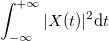 .
.
According to the Plancherel theorem: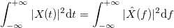 .
.
Average power function on the segment  defined as
 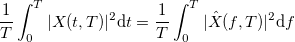 .
.
Then the power spectral density is:

If the length of the segment tends to infinity, then:
 .
.
Since function describes the FBD with the Hirst parameter , then:
FFT discrete transform
The FBD modeling process can be simplified through the approximation of the Fourier transform using Fourier series, taking into account the conservation of the properties of the spectral density. After that, using the inverse Fourier transform, we obtain FBD.
If a

that function real-valued.
Thus, the algorithm below uses this condition of conjugate symmetry.
Algorithm for constructing a FBD curve:
 - a normally distributed random variable with zero expectation mat and unit standard deviation.
 - uniformly distributed random variable on a unit segment.
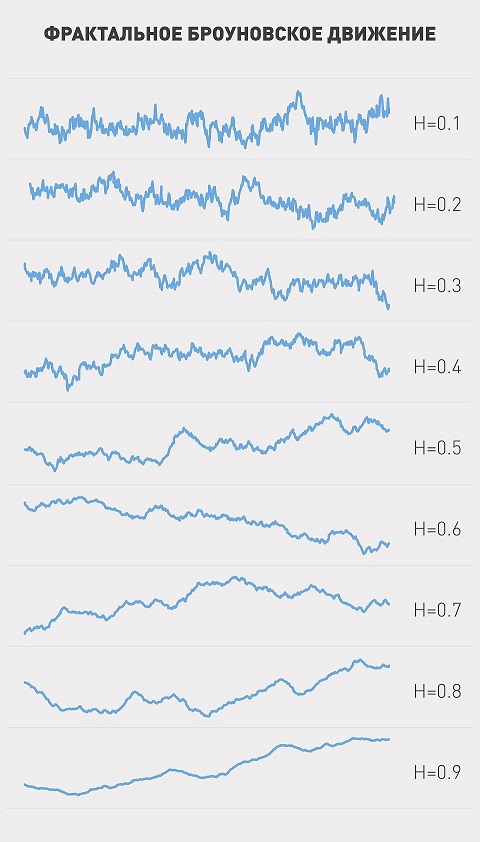
The figure shows some variations of the FWD for different indicators of Hirst.
FWA generation usage example
Given the original series of the currency pair dollar-ruble for the period: 05.05.2005 - 01.05.2015.
We calculate the exchange rate yields and, using RS analysis, find the Hurst index for the dollar-ruble pair: H = 0.64 is separated from the mean value E (H) = 0.52 by 5.64 standard deviations. The value of H is significant. The row is persistent, since H> 0.5 , the normalized scale changes the scale faster than the square root in time, the process has a long-term memory (more details in [1]).
The absence of a cycle allows, using the Hirst parameter, to model the fractal noise using Fourier filtering. In the frequency domain, we construct the Fourier transform of fractal Brownian motion with random amplitudes and phases satisfying the spectral density property. C using the inverse Fourier transform we obtain the desired fractal noise.
Next, we generate 10,000 various variations of the FWA with the Hurst index of 0.64. Thus we obtain the distribution of forecast values for the exchange rate.
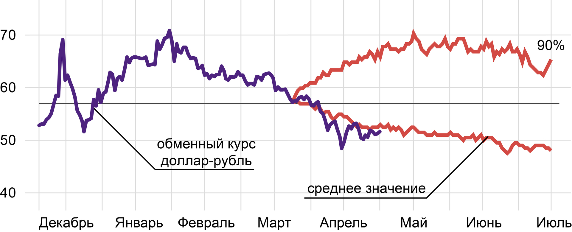
The figure shows a graph of the original series of dollar-ruble exchange rates, and 90% is the distribution decile and expected expectation: with a 90% probability, it can be argued that the rate will not exceed the values of the upper curve, the average exchange rate has a downward trend; the average price per dollar will be 52.3 rubles, the beginning of June - 51.6, the beginning of July - the price will drop to the level of 48.7 rubles.
Bibliography:
,where is the function
, satisfies the condition: Fourier transform
For FWD, we will interpret the process
as a time process. There is a frequency domain in which the function is the sum of the components having a certain frequency. Function can be decomposed as .Component
with frequency has the form: where .')
Function
called the Fourier transform .Spectral density
The total energy of the original process is
.According to the Plancherel theorem:
.Average power function
on the segment defined as .Then the power spectral density is:
If the length of the segment tends to infinity, then:
.Since function
describes the FBD with the Hirst parameter , then:FFT discrete transform
The FBD modeling process can be simplified through the approximation of the Fourier transform using Fourier series, taking into account the conservation of the properties of the spectral density. After that, using the inverse Fourier transform, we obtain FBD.
If a
that function
real-valued.Thus, the algorithm below uses this condition of conjugate symmetry.
Algorithm for constructing a FBD curve:
- a normally distributed random variable with zero expectation mat and unit standard deviation. - uniformly distributed random variable on a unit segment.
- For
 Fourier Transform Values
- For
 -
- 
- For each
 calculate: amplitude (the absolute value of the complex number
  ), phase (the value of the argument of a complex number i.e. angle, expressed in radians)
 - Calculate the values of the FWD:

The figure shows some variations of the FWD for different indicators of Hirst.
FWA generation usage example
Given the original series of the currency pair dollar-ruble for the period: 05.05.2005 - 01.05.2015.
We calculate the exchange rate yields and, using RS analysis, find the Hurst index for the dollar-ruble pair: H = 0.64 is separated from the mean value E (H) = 0.52 by 5.64 standard deviations. The value of H is significant. The row is persistent, since H> 0.5 , the normalized scale changes the scale faster than the square root in time, the process has a long-term memory (more details in [1]).
The absence of a cycle allows, using the Hirst parameter, to model the fractal noise using Fourier filtering. In the frequency domain, we construct the Fourier transform of fractal Brownian motion with random amplitudes and phases satisfying the spectral density property. C using the inverse Fourier transform we obtain the desired fractal noise.
Next, we generate 10,000 various variations of the FWA with the Hurst index of 0.64. Thus we obtain the distribution of forecast values for the exchange rate.
The figure shows a graph of the original series of dollar-ruble exchange rates, and 90% is the distribution decile and expected expectation: with a 90% probability, it can be argued that the rate will not exceed the values of the upper curve, the average exchange rate has a downward trend; the average price per dollar will be 52.3 rubles, the beginning of June - 51.6, the beginning of July - the price will drop to the level of 48.7 rubles.
Bibliography:
- Goncharenko A.V. Fractal analysis of the dynamics of the USD / RUB currency pair // Risk management in a credit institution. №2 (18). 2015. p. 18-22.
Source: https://habr.com/ru/post/257409/
All Articles